TensorRT-LLM 源码完全拆解(十一):并行拓扑与通信——Mapping、DeviceMesh 与 Communicator 如何组织一次多卡前向
从这一篇开始进入通信与并行主线
这个系列此前走完了 TensorRT-LLM 的调度、KV Cache 管理与注意力后端:调度器如何准入请求(可参考 TensorRT-LLM 源码完全拆解(三):调度器内部),KV 块如何记物理账(可参考 TensorRT-LLM 源码完全拆解(四):KVCacheManager 与块管理),注意力后端如何把块句柄翻成索引数组(可参考 TensorRT-LLM 源码完全拆解(六):Attention Backend 的 prepare() 内部)。
这些机制都有一个共同的前提:一次前向并不发生在一张卡上。当模型被切到 8 张、64 张甚至上千张 GPU 上时,每一层的矩阵乘都只算了一部分,必须靠集合通信把碎片拼回完整结果。调度器看到的”一个 batch”,实际上是几十个 rank 上同时发生的一组本地计算加上一组互相等待的通信操作。
这一篇要回答三个问题:
- rank 坐标系怎么建:
Mapping如何把一个全局 rank 编号翻译成(pp_rank, tp_rank, cp_rank, moe_tp_rank, moe_ep_rank)这样一组坐标,并据此划分出各类通信组; - 进程组怎么落地:MPI 编排和 Ray(DeviceMesh)编排两种模式下,逻辑上的通信组如何变成 PyTorch 的
ProcessGroup,以及两种模式的语义差异; - 通信本身怎么优化:
Communicator抽象背后的数据面——NCCL、自定义 one-shot/two-shot kernel、MNNVL 多播、对称内存 MULTIMEM、低精度传输,各自在什么拓扑下被选中。
第 3 点尤其重要,因为 TensorRT-LLM 真正的性能优势有很大一部分不在 GEMM 里,而在把 GEMM 和 all-reduce 融合成一次访存这件事上。这一篇会把这条路径上的取舍讲清楚。
背景:为什么需要一张”并行拓扑表”
先回到最基础的问题。张量并行(Tensor Parallel,TP)的做法是把一个线性层的权重矩阵按列或按行切开,每张卡只存一份切片。以 Transformer 里最常见的 QKV 投影 + 输出投影 这一对为例:
- 列并行(column parallel):权重按输出维度切分,,每张卡算出输出的一部分 。输出不完整,需要
all-gather才能拼回完整的 。 - 行并行(row parallel):权重按输入维度切分,每张卡拿到的是 的一部分 ,算出的是部分和 。要让每张卡都拿到完整结果,需要
all-reduce:。
标准做法是”列并行接行并行”:QKV 投影用列并行(不需要立刻通信,因为注意力可以按头切分,各卡只算自己那几个头的注意力),输出投影用行并行(结束时一次 all-reduce 把部分和加起来)。这样每层的通信次数是 1 次 all-reduce。
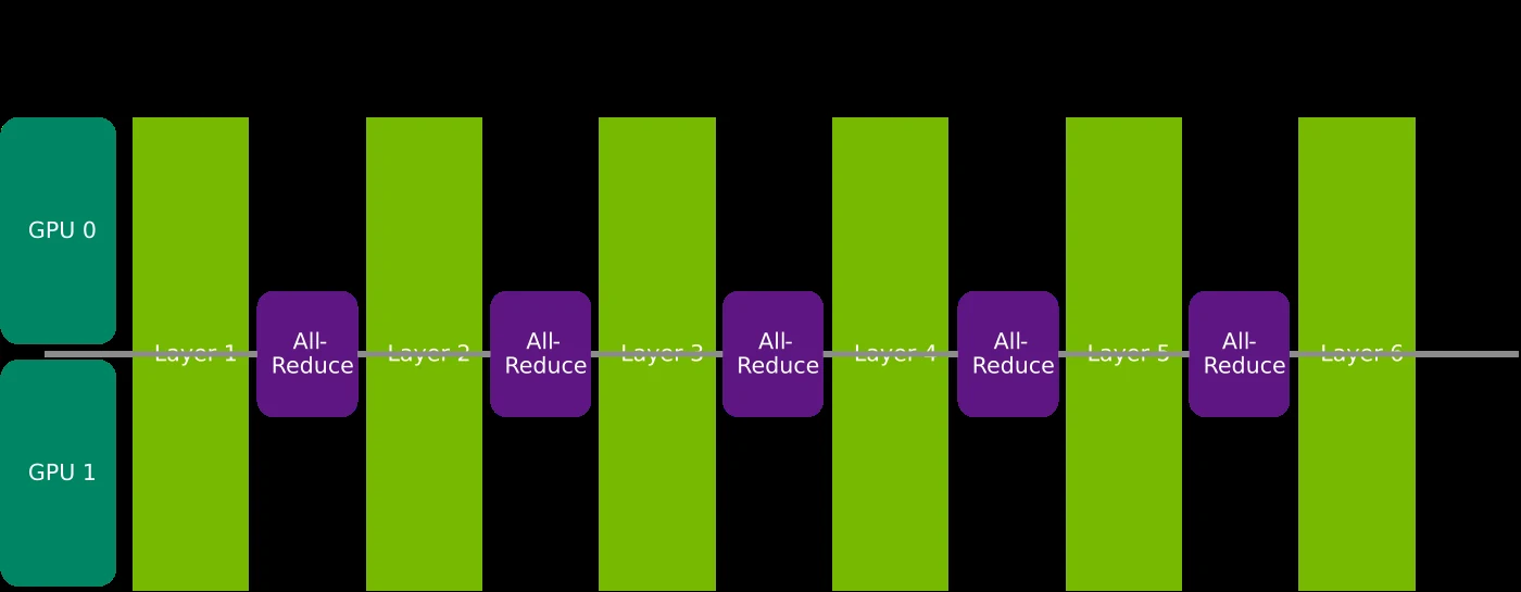
图源:TensorRT-LLM 官方文档(docs/source/media/Tensor_Parallelism_Vis.svg)。
于是通信就成了关键路径。以 Llama-3-70B 为例,hidden size 8192、80 层、bf16 权重,每层的 all-reduce 要搬运 字节( 是 token 数)。当 batch 很小、decode 阶段每步只有几百个 token 时,GEMM 本身只要几十微秒,而 all-reduce 的固定延迟(NCCL 起步约 5–20 µs,加上 kernel launch 和同步开销)占比就非常可观。
这就带来两个工程命题:
- 拓扑必须被精确描述:不同并行策略(TP、PP、CP、MoE 的 TP/EP/cluster、attention DP)需要的通信组完全不同。一张卡在 TP 组里是 rank 3,在 PP 组里可能是 rank 0,在 MoE EP 组里又是另一个位置。如果没有一张明确的”拓扑表”,代码里到处都会是手写的 rank 算术,没法维护。
- 通信必须被极致优化:常规 NCCL all-reduce 在 NVLink 域内已经很快,但它仍然是”写一次、读一次、再写一次”的额外访存。如果能把这个搬运省掉,或者和归一化、量化算子融合到一起,收益比调 GEMM 的 tile 更大。
TensorRT-LLM 的答案分别是 tensorrt_llm/mapping.py(拓扑表)和 tensorrt_llm/_torch/distributed/(通信层)。
Mapping:一张卡的身份坐标
Mapping 是 TensorRT-LLM 里所有并行逻辑的入口。它的构造签名(tensorrt_llm/mapping.py)本身就是一份并行策略清单:
def __init__(self, world_size=1, rank=0, gpus_per_node=8, *, cp_size=1, cp_config=None, tp_size=1, pp_size=1, pp_partition=None, moe_cluster_size=-1, moe_tp_size=-1, moe_ep_size=-1, attn_tp_size=-1, attn_cp_size=-1, enable_attention_dp=False, enable_lm_head_tp_in_adp=False, dwdp_size=0, dwdp_rank=0):参数分成四类,理解这个分类是读懂后面所有代码的前提:
| 类别 | 参数 | 含义 |
|---|---|---|
| 全局 | world_size、rank、gpus_per_node | 这次作业一共几张卡、我是第几张、单机几张 |
| 主并行 | tp_size、pp_size、cp_size | 张量并行、流水并行、上下文并行 |
| MoE 并行 | moe_cluster_size、moe_tp_size、moe_ep_size | 专家的分组/张量/专家并行维度 |
| 注意力特殊布局 | attn_tp_size、attn_cp_size、enable_attention_dp | 注意力层单独使用的 TP/CP 切法 |
| 权重分布式数据并行 | dwdp_size、dwdp_rank | DWDP,专家权重的冗余副本维度 |
第一层校验:主并行的乘法关系
构造函数里最先做的是一组硬校验。最关键的一条是:
if tp_size * pp_size * cp_size != world_size: raise ValueError( "world_size must equal to tp_size * pp_size * cp_size, " f"but got {world_size} != {tp_size} * {pp_size} * {cp_size}.")这条约束把 TP、PP、CP 定义为正交的三个维度,三者相乘恰好覆盖全部 rank,不允许重叠也不允许留空。原因在于后面所有组划分都基于”全局 rank 号做一个混合进制分解”:
这条公式直接对应 MpiTopology 里的三个 property:
@propertydef tp_rank(self) -> int: return self.rank % (self.tp_size * self.cp_size) // self.cp_size
@propertydef pp_rank(self) -> int: return self.rank // (self.tp_size * self.cp_size)
@propertydef cp_rank(self) -> int: return self.rank % self.cp_size用大白话讲:PP 是最高位、TP 是中间位、CP 是最低位。全局 rank 先按 PP 分段,段内再按 TP 分段,每段内连续的 cp_size 个 rank 是同一个 CP 组。
顺序不是随便定的,它决定了通信组在物理拓扑上是否连续。CP 放在最低位意味着一个 CP 组是连续编号的 rank,能落在同一台机器内部的连续 GPU 上;TP 组则是步长为 cp_size 的交错 rank 集合。
Mapping 的 docstring 给了几个具体例子,值得逐个对照:
A node with 8 GPUs, tp_size = 4, cp_size = 1, pp_size = 2
2 tp groups:- [0, 1, 2, 3]- [4, 5, 6, 7]
4 pp groups:- [0, 4]- [1, 5]- [2, 6]- [3, 7]tp_size=4, cp_size=1, pp_size=2,world_size=8。按公式,tp_rank = rank % 4,pp_rank = rank // 4。rank 0–3 是 pp_rank 0,rank 4–7 是 pp_rank 1。TP 组是同一 pp_rank 内所有 rank,所以是 [0,1,2,3] 和 [4,5,6,7];PP 组是”相同 tp_rank、不同 pp_rank”,即 [0,4]、[1,5]……
再看 CP 非 1 的情况:
A node with 8 GPUs, tp_size = 4, cp_size = 2, pp_size = 1
4 cp groups:- [0, 1]- [2, 3]- [4, 5]- [6, 7]
2 tp groups:- [0, 2, 4, 6]- [1, 3, 5, 7]这里 CP 组是连续对 [0,1],TP 组变成步长 2 的交错集 [0,2,4,6]。这正是”CP 放最低位”的直接后果。把 CP 放在最低位,是为了让上下文并行组内的通信走机内 NVLink——CP 的通信量(每个 token 的所有 KV)远大于 TP 的通信量(每个 token 的 hidden state),更需要高带宽域。
第二层:MoE 并行的三重复合关系
MoE 层的并行比稠密层复杂得多。Mapping 里与 MoE 相关的字段有四个,彼此之间还有一个必须成立的等式:
moe_world_size = tp_size if cp_type == CpType.ULYSSES else tp_size * cp_size
moe_tp_ep_size = moe_tp_size * moe_ep_sizeself.moe_tp_cluster_ep_size = moe_tp_ep_size * moe_cluster_sizeif not (dwdp_size > 1) and self.moe_tp_cluster_ep_size != moe_world_size: raise ValueError( "moe_tp_size * moe_ep_size * moe_cluster_size must equal to moe_world_size, " f"but got {self.moe_tp_cluster_ep_size} != {moe_world_size}")即
为什么必须相等?因为专家的总张量副本数是被并行度整除的关系决定的。一个 MoE 层共有 个专家,如果 moe_ep_size = 8,那么每个 rank 只装 个专家。同时 moe_tp_size 又把每个专家自己的权重切开,moe_cluster_size 则是把若干相邻的 EP 组捆成一个”cluster”(用于让一个 token 在 cluster 内部就能找到它需要的所有专家,从而避免跨 cluster 的 all-to-all)。三个维度各自乘起来,必须等于”所有参与 MoE 计算的 rank 数”——否则专家的账目对不上。
注意 moe_world_size 的取值依赖 cp_type:ULYSSES 模式下 CP 与 TP 是”同一批物理卡上的两种视角”,所以 MoE 的世界大小等于 tp_size;而 HELIX 模式下 CP 的这批 rank 在 FFN 层会被重新用作 TP(见后面的 repurpose_helix_cp_to_tp),所以 MoE 世界大小扩到 tp_size * cp_size。
第三层:注意力层的独立切法
attn_tp_size 和 attn_cp_size 是 TensorRT-LLM 里比较特殊的一组参数。它们的约束是:
attn_tp_cp_size = attn_tp_size * attn_cp_sizeif attn_tp_cp_size != tp_size * cp_size: raise ValueError( "tp_size * cp_size must equal to attn_tp_size * attn_cp_size, ...")
if attn_cp_size != 1 and cp_type == CpType.ULYSSES: raise ValueError( f"attn_cp_size must be 1 for now for ulysses, but got {attn_tp_size}, {attn_cp_size}.")含义是:注意力层可以把 TP 和 CP 的”合并维度”重新分配。总容量 不变,但其中多少用于 TP、多少用于 CP 可以由注意力层自己决定。这在 HELIX 模式下很有用——当 cp_size=8, tp_size=1 时,注意力层可以把 attn_cp_size 设得小一些、attn_tp_size 设得大一些,让注意力也吃到张量并行的好处。
ULYSSES 模式不允许 attn_cp_size != 1,因为 Ulysses 的 CP 是”按 head 维度切分再 all-to-all”的经典实现,其通信组与 TP 组是同一个物理集合的不同视图,把 CP 再拆开就失去了意义。
组划分:MpiTopology._init_parallel_groups
MappingBase.__init__ 只负责校验和保存标量;真正的组划分发生在 MpiTopology._init_parallel_groups(mapping.py)。它是一段非常值得逐行读的代码,因为它用四条 range 表达式把前面那张拓扑表全部实现了:
def _init_parallel_groups(self): # init pp group for i in range(self.tp_size * self.cp_size): ranks = range(i, self.world_size, self.tp_size * self.cp_size) self.pp_groups.append(list(ranks))
# init cp group (consecutive ranks within each tp slice). for i in range(self.pp_size): for j in range(self.tp_size): ranks = range( i * self.tp_size * self.cp_size + j * self.cp_size, i * self.tp_size * self.cp_size + (j + 1) * self.cp_size) self.cp_groups.append(list(ranks))
# init tp group (interleaved ranks with stride of cp_size). for i in range(self.pp_size): for j in range(self.cp_size): ranks = range(i * self.tp_size * self.cp_size + j, (i + 1) * self.tp_size * self.cp_size + j, self.cp_size) self.tp_groups.append(list(ranks))逐个理解:
PP 组:步长是 tp_size * cp_size,起点从 0 到 tp_size * cp_size - 1。这就是”固定 (tp_rank, cp_rank),扫过所有 pp_rank”。共有 tp_size * cp_size 个 PP 组。
CP 组:在每个 (pp_rank, tp_rank) 组合下,取一段长度为 cp_size 的连续区间。共有 pp_size * tp_size 个 CP 组。
TP 组:在每个 (pp_rank, cp_rank) 组合下,从 i * tp_size * cp_size + j 开始,以 cp_size 为步长走到该 PP 段的末尾。共有 pp_size * cp_size 个 TP 组。
三段代码和前面 tp_rank/pp_rank/cp_rank 的公式完全自洽。以 8 卡、tp=4, cp=2, pp=1 为例验证一下 CP 组:
i = 0(pp_rank 0),j从 0 到 3:j=0:range(0*8 + 0*2, 0*8 + 1*2)=[0, 1]j=1:range(0 + 2, 0 + 4)=[2, 3]j=2:[4, 5],j=3:[6, 7]
得到 4 个 CP 组 [0,1] [2,3] [4,5] [6,7],与 docstring 一致。
MoE 组的划分:为什么索引表达式这么长
MoE 的那三段循环索引表达式看起来吓人,但只要记住 “MoE 世界是三层嵌套:cluster 在外、EP 在中、TP 在内” 就能读懂:
# init moe tp groupfor i in range(self.pp_size): for j in range(self.moe_cluster_size * self.moe_ep_size): ranks = range(i * self.moe_tp_cluster_ep_size + j, (i + 1) * self.moe_tp_cluster_ep_size, self.moe_cluster_size * self.moe_ep_size) self.moe_tp_groups.append(list(ranks))MoE TP 组:固定 (pp_rank, moe_cluster_rank, moe_ep_rank),扫过 moe_tp_size 个 rank,步长是 moe_cluster_size * moe_ep_size。也就是”同一份专家权重切片在不同 TP 分片上的那些卡”。
# init moe ep groupfor i in range(self.pp_size): for j in range(self.moe_tp_size): for k in range(self.moe_cluster_size): ranks = range( i * self.moe_tp_cluster_ep_size + j * self.moe_cluster_size * self.moe_ep_size + k * self.moe_ep_size, i * self.moe_tp_cluster_ep_size + j * self.moe_cluster_size * self.moe_ep_size + (k + 1) * self.moe_ep_size) self.moe_ep_groups.append(list(ranks))MoE EP 组:固定 (pp_rank, moe_tp_rank, moe_cluster_rank),取连续的一段 moe_ep_size 个 rank。这是 all-to-all 通信真正走的组——每个 rank 把自己的 token 按路由结果发给同 EP 组内的其他 rank,再把收到的 token 算完发回去。
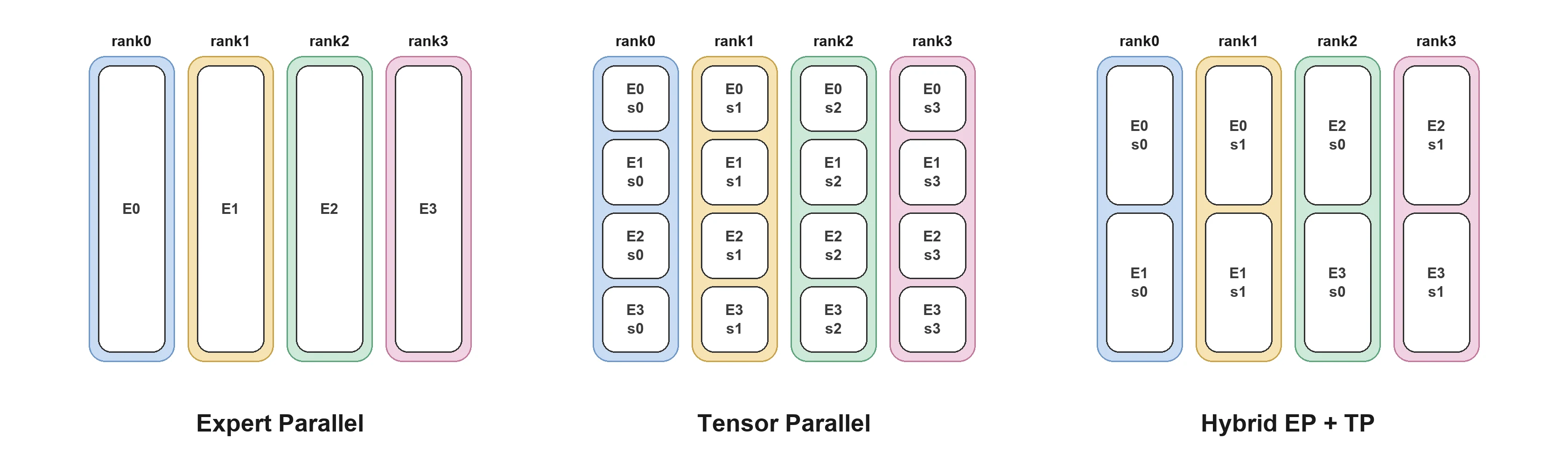
图源:TensorRT-LLM 官方文档(docs/source/media/moe-parallelism.png)。专家维度(EP)决定”哪些专家放在哪个 rank 上”,张量维度(TP)决定”每个专家自己的权重再切成几份”。图里几组配置的对比正是后面那条 moe_tp_size × moe_ep_size × moe_cluster_size = moe_world_size 等式的图解。
对照 docstring 的例子验证 moe_tp_size = 2, moe_ep_size = 4(8 卡):
- MoE TP 组:
j从 0 到moe_cluster_size(1) * moe_ep_size(4) - 1 = 3,步长 4,长度 8。j=0得[0, 4],j=1得[1, 5],j=2得[2, 6],j=3得[3, 7]。4 个组,与 docstring 一致。 - MoE EP 组:
j只有 0(moe_tp_size=2→ j 取 0,1;但moe_cluster_size=1时 j 循环的是moe_tp_size),k=0,得range(0, 4)=[0,1,2,3];j=1得range(4, 8)=[4,5,6,7]。2 个组,与 docstring 一致。
属性的取值索引也是精心设计的
有了组列表之后,每个 rank 要能”取出自己所属的那个组”。MpiTopology 靠的是与组生成顺序严格对应的索引公式:
@propertydef cp_group(self) -> List[int]: return self.cp_groups[self.pp_rank * self.tp_size + self.tp_rank]
@propertydef tp_group(self) -> List[int]: return self.tp_groups[self.pp_rank * self.cp_size + self.cp_rank]
@propertydef pp_group(self) -> List[int]: return self.pp_groups[self.tp_rank * self.cp_size + self.cp_rank]这三个索引公式和上面三个生成循环的循环变量顺序是一一对应的:cp_groups 是 (i=pp_rank, j=tp_rank) 双层循环,所以索引是 pp_rank * tp_size + tp_rank;tp_groups 是 (i=pp_rank, j=cp_rank),所以是 pp_rank * cp_size + cp_rank;pp_groups 只有一层且以”固定的 (tp_rank, cp_rank)”为准,所以是 tp_rank * cp_size + cp_rank。
MoE 的三个 group 索引同理,只是层级更深:
@propertydef moe_ep_group(self) -> List[int]: return self.moe_ep_groups[self.pp_rank * self.moe_tp_size * self.moe_cluster_size + self.moe_tp_rank * self.moe_cluster_size + self.moe_cluster_rank]这类”生成顺序 = 索引公式”的写法在分布式代码里很常见,也很容易写错。读这段代码时最实用的方法是:先在纸上写出组列表的遍历顺序树,再去核对 property 里的乘法权重。
repurpose_helix_cp_to_tp:HELIX 模式的”身份切换”
HELIX 上下文并行有一条独特的设计:CP 只对注意力层有意义,到了 FFN/MoE 层,这批 rank 被重新当成 TP 用。代码里体现为一个方法:
def repurpose_helix_cp_to_tp(self): # In helix parallelism, CP is relevant only for the attention layer. # These ranks are repurposed to TP for FFN layers. assert self.has_cp_helix() return Mapping( world_size=self.world_size, rank=self.rank, gpus_per_node=self.gpus_per_node, cp_size=1, cp_config={}, tp_size=self.tp_size * self.cp_size, pp_size=self.pp_size, ... )它返回一个新的 Mapping 对象:cp_size 归零,tp_size 变成原来的 tp_size * cp_size。也就是说,同一张卡在同一个模型里持有两个 Mapping——注意力层用前者,FFN 层用后者。这不是”改配置”,而是同一批硬件上两种不同的逻辑视图,这也是 HELIX 能把 CP 的通信开销摊薄的原因:CP 期间被切开的卡,在 FFN 期间全部拿去做 TP,算力不浪费。
张量并行的权重切分:从 Mapping 到 Linear
拓扑表建好了,具体到每一层怎么切权重?tensorrt_llm/_torch/modules/linear.py 里的 TensorParallelMode 只有两个取值,却定义了整套切分语义:
class TensorParallelMode(str, enum.Enum): COLUMN = 'column' ROW = 'row'
@classmethod def split_dim(cls, mode): return 1 if mode == cls.ROW else 0
# Helper to shard the corresponding per-channel activation scales # which are sharded along the dimension orthogonal to the weights @classmethod def flip(cls, mode): return cls.ROW if mode == cls.COLUMN else cls.COLUMNsplit_dim 给出的是权重矩阵的切分维度:COLUMN 切 dim 0(输出维),ROW 切 dim 1(输入维)。flip 则是给量化 per-channel scale 用的——scale 的切分维度与权重正交,所以要从 COLUMN 翻成 ROW、从 ROW 翻成 COLUMN。这个细节在很多手写 TP 实现里会被忽略,结果是 scale 和权重错位,数值悄悄出错。
Linear.__init__ 里保存的 self.tp_mode、self.tp_rank、self.tp_size 全部来自 Mapping,切分本身在权重加载阶段完成(load_shard)。真正与通信相关的是 forward:
def forward(self, input, *, all_reduce_params=None, lora_params=None, layer_idx=None): if self.tp_mode == TensorParallelMode.ROW: ... bias = None if (self.tp_rank > 0) else self.bias if self.reduce_output: if use_fused_gemm_allreduce: output = self.apply_linear_allreduce(input, self.bias, layer_idx) else: ... use_nccl_symmetric_memory_window = (...) output = self.all_reduce(output, all_reduce_params=all_reduce_params) else: output = self.apply_linear(input, bias, lora_params, layer_idx) elif self.tp_mode == TensorParallelMode.COLUMN: output = self.apply_linear(input, self.bias, lora_params, layer_idx) if self.gather_output: from ..distributed import allgather output = allgather(output, self.mapping, sizes=self.gather_output_sizes) else: output = self.apply_linear(input, self.bias, lora_params, layer_idx) return output三条分支对应三件事,值得逐一说明:
- ROW +
reduce_output:算完之后 all-reduce。这是主干路径,也是后面所有”融合”优化的落点。注意bias = None if self.tp_rank > 0 else self.bias——bias 只在 rank 0 上加,因为 all-reduce 会把各 rank 的部分和相加,如果每张卡都加一遍 bias,最终结果会多出tp_size份。这是个很容易写错的细节。 - COLUMN +
gather_output:算完之后 all-gather。但 Transformer 里几乎不用它——列并行的输出通常直接喂给下一层,不需要拼回完整张量;只有需要完整输出的地方(比如 LM head 之后再切)才用。 - 无 tp_mode:权重不切,纯本地计算。
还有一行容易被忽略的逻辑:
self.gather_output_sizes = Noneif self.gather_output and self.tp_size > 1 \ and self.tp_mode == TensorParallelMode.COLUMN: if self._tp_sharding_is_auto: sizes = [end - start for start, end in ...] ... self.gather_output_sizes = sizesallgather 带 sizes 参数是为了支持不均匀切分(uneven TP)——当输出维度不能被 tp_size 整除时,各 rank 分到的宽度不同,all-gather 必须显式知道每段的长度,否则按等长拼接会错位。
DeviceMesh:Ray 模式下如何用 PyTorch 原生机制表达同一张拓扑表
前面讲的 MpiTopology 是 MPI 编排模式下的实现。TensorRT-LLM 同时支持 Ray 编排(多实例、弹性扩缩场景),这时 Mapping 会走另一条路:
def __new__(cls, *args, **kwargs): if mpi_disabled(): return super().__new__(DeviceMeshTopology) else: return super().__new__(MpiTopology)Mapping 用 __new__ 做了一个运行期分派:MPI 可用时是 MpiTopology,否则是 DeviceMeshTopology。注意 DeviceMeshTopology 同时继承 DeviceMeshTopologyImpl 和 Mapping,前者的 tp_rank / tp_group 等属性会覆盖后者的实现。
DeviceMeshTopologyImpl.build_mesh(tensorrt_llm/_torch/device_mesh.py)用 PyTorch 的 init_device_mesh 一次性建出多维网格:
def build_mesh(self): cls = DeviceMeshTopologyImpl if self.world_size == 1 or cls.device_mesh is not None: return # only build mesh once ... # Dimensions go from slowest-varying (outermost) to fastest-varying (innermost). # Layout: pp is outermost, then tp, then cp is innermost (consecutive). dims = ["pp"] shape = [self.pp_size]
if self.moe_ep_size > 1: dims += ["moe_tp", "moe_ep"] shape += [self.moe_tp_size, self.moe_ep_size] else: dims += ["tp"] shape += [self.tp_size]
dims += ["cp"] shape += [self.cp_size]
cls.device_mesh = init_device_mesh( "cuda", mesh_shape=tuple(shape), mesh_dim_names=tuple(dims), )
if self.moe_ep_size > 1: cls.tp_mesh = cls.device_mesh["moe_tp", "moe_ep"]._flatten(mesh_dim_name="tp")这段代码里藏着三个重要设计:
第一,维度顺序被显式声明为”从最慢变化到最快变化”:pp 在最外、cp 在最内。这与前面 rank = pp_rank * (tp*cp) + tp_rank * cp + cp_rank 的分解完全一致——DeviceMesh 的 mesh_shape 展平时,最后一个维度变化最快,对应的正是 rank 的最低几位。两种编排模式下 rank 的语义因此保持一致,上层模型代码不需要区分。
第二,MoE 与稠密走不同的维度命名:当 moe_ep_size > 1 时,TP 维度被替换成 ["moe_tp", "moe_ep"] 两维,形状是 [moe_tp_size, moe_ep_size]。这两维的乘积恰好是原来的 tp_size(在 cp_type != HELIX 且 moe_cluster_size == 1 的情形下)。这解释了前面那条等式约束——不是”为了好看”,而是网格形状必须能精确表示 rank 空间。
第三,tp_mesh 是 MoE 两维的展平:
cls.tp_mesh = cls.device_mesh["moe_tp", "moe_ep"]._flatten(mesh_dim_name="tp")MoE 场景下稠密层的 TP 组需要跨越 moe_tp 和 moe_ep 两个维度(因为这两维合起来才是全量的 rank 空间),所以代码把它们展平成一个叫 tp 的虚拟维度。取用时的分派逻辑在 _get_mesh_dim_by_name:
def _get_mesh_dim_by_name(self, name): if self.world_size == 1: return SingleProcessGroup() if name == 'tp': if 'tp' in cls.device_mesh.mesh_dim_names: return cls.device_mesh['tp'] else: return cls.tp_mesh else: assert name in cls.device_mesh.mesh_dim_names, ... return cls.device_mesh[name]以及一个必须处理的退化情形:
if self.world_size == 1: # A single-rank mapping reports rank 0 of a size-1 group for every # dimension, whatever mesh the job built: the mesh belongs to the # job, not to this mapping. return SingleProcessGroup()注释点出了一个真实的问题:DeviceMesh 是进程级的全局单例(cls.device_mesh),一旦建好就属于整个作业;而 Mapping 是每个 LLM 实例自己的配置。当同一个进程里跑了一个 world_size=1 的 Mapping(比如做单卡测试或跑一个小的辅助模型)时,不能让它去用作业级的网格,否则会拿到错误的 group。SingleProcessGroup(device_mesh.py)就是为此准备的哨兵对象,它伪造出 rank=0、size=1 的接口。
DeviceMeshTopologyImpl 的各个 rank 属性也都改成了向网格问:
@propertydef tp_rank(self) -> int: return self.tp_group_pg.rank()
@propertydef cp_rank(self) -> int: return self.cp_group_pg.rank()也就是说,MPI 模式下 rank 坐标是算出来的(对全局 rank 做混合进制分解),DeviceMesh 模式下 rank 坐标是问出来的(问 ProcessGroup 自己在组内的序号)。两种实现必须给出相同的结果,否则同一个模型在两种编排下会有不同的行为。这是读这段代码时值得注意的”契约”。
小结(上):拓扑表的设计要点
到这里可以把上半篇的结论收拢:
Mapping的核心是一个混合进制 rank 分解:rank = pp_rank × (tp×cp) + tp_rank × cp + cp_rank。CP 放在最低位是为了让 CP 组连续、落在机内 NVLink 域。- 三条等式约束定义了整个并行空间的合法性:
tp × pp × cp = world_size、moe_tp × moe_ep × moe_cluster = moe_world_size、attn_tp × attn_cp = tp × cp。违反任何一条都会在构造时直接抛错,不会留到运行期才炸。 - 组划分与组索引是两段必须成对阅读的代码:四个
_init_parallel_groups循环决定了组列表的排列顺序,property 里的乘法权重必须与之严格对应。 repurpose_helix_cp_to_tp展示了 HELIX 的本质:同一批卡在注意力层当 CP、在 FFN 层当 TP,一个进程持有两个 Mapping。- Ray 模式用
init_device_mesh复刻同一套语义:维度顺序[pp, (moe_tp, moe_ep) | tp, cp]与 MPI 的 rank 分解一致,MoE 的两维被展平成虚拟tp维度。 Linear.forward是拓扑落到算子上的地方:ROW 型末尾 all-reduce(bias 只在 rank 0 加)、COLUMN 型可选 all-gather(支持不均匀切分时需显式sizes)。
下一节进入数据面:这些组之上的通信到底怎么发出去。
通信层的两种编排:MPIDist 与 TorchDist
tensorrt_llm/_torch/distributed/communicator.py 定义了通信层的抽象基类 Distributed。它的设计意图很明确:上层模型代码只调用语义化的通信原语,不关心底层是 MPI 还是 NCCL。
class Distributed(ABC):
def __init__(self, mapping: Mapping): self.mapping = mapping
@staticmethod @lru_cache(maxsize=None) def get(mapping: Mapping) -> "Distributed": if mpi_disabled(): return TorchDist(mapping) else: return MPIDist(mapping)Distributed.get 用 lru_cache 缓存,键是 Mapping 对象本身。这要求 Mapping 实现了 __hash__(MappingBase.__hash__ 把一组标量字段编成一个元组哈希),否则缓存会失效甚至报错。缓存的意义在于:模型里每个 Linear 层都会调用 Distributed.get(mapping) 拿通信对象,如果每次都新建就会重复建立进程组。
MPIDist:把 MPI 当通信后端
MPIDist 直接持有 MPI 通信子:
class MPIDist(Distributed): tp_comm: MPI.Comm
def __init__(self, mapping: Mapping): super().__init__(mapping) self._cp_comm = None self._tp_comm = None self._pp_comm = None
def _validate_world_size(self): """Validate world size before creating sub-communicators to prevent segfaults.""" if ENABLE_MULTI_DEVICE: actual_world_size = mpi_world_size() max_rank_needed = self.mapping.world_size if max_rank_needed > actual_world_size: raise RuntimeError( f"Mapping requires world_size={max_rank_needed} " f"(tp_size={self.mapping.tp_size} * pp_size={self.mapping.pp_size} * cp_size={self.mapping.cp_size}), " f"but MPI world size is only {actual_world_size}. ")_validate_world_size 的存在理由写在注释里——在建子通信子之前先校验,否则会 segfault。这是分布式编程里最经典的踩坑点:MPI_Comm_split 之类的调用如果 rank 数对不上,行为是未定义的,很多 MPI 实现直接崩掉而不是返回错误。把一个”配置错误”翻译成一次段错误,排查成本极高,所以这里宁可显式抛异常。
通信组按需延迟创建,三个 _*_comm 初始都是 None:
@propertydef tp_comm(self): ...@propertydef cp_comm(self): ...@propertydef pp_comm(self): ...只有真正用到某个维度的通信时才建对应的子通信子。这带来的好处是:如果一个作业里 CP 从不使用(cp_size=1),就永远不会创建 CP 通信子,也就不会有它的建组开销。
TorchDist:Ray 模式下的初始化顺序
Ray 模式下没有 MPI,通信后端是 PyTorch 原生的 torch.distributed。TorchDist.__init__ 藏着一段顺序关键的逻辑:
def __init__(self, mapping: Mapping): super().__init__(mapping) assert dist.is_initialized( ), "torch.distributed should be initialized before TorchDist"
self.cluster_info = None
from tensorrt_llm._utils import set_torch_comm set_torch_comm(self) # Set as global instance mapping.build_mesh()
self.setup_local_comm() self.default_store = torch.distributed.distributed_c10d._get_default_store()
init_pg(torch.distributed.group.WORLD, self.local_comm, torch_pybind11_abi())四个步骤,每一步都有理由:
set_torch_comm(self):把自己注册成全局单例。C++ 侧的 custom op(比如torch.ops.trtllm.allreduce_pg)在没有 MPI 时需要通过这个全局引用回拿通信对象。mapping.build_mesh():建 DeviceMesh。这一步必须在建 local comm 之前,因为DeviceMeshTopology的tp_group_pg等属性依赖网格。setup_local_comm():按节点划分本地通信组。init_pg(...):把 WORLD 组和 local 组的句柄传给 C++ 侧的进程组管理器(init_pg),让 custom op 能直接拿到ProcessGroup。
setup_local_comm 的实现值得细看:
def setup_local_comm(self): self._get_cluster_info()
# node IP -> list of ranks ip_to_ranks = {} for rank, (node_ip, _) in enumerate(self.cluster_info): ip_to_ranks.setdefault(node_ip, []).append(int(rank))
self.local_comm = None for ranks in ip_to_ranks.values(): # All global ranks from the default process group to participate in the call, # even if some ranks are not part of the new process group being created pg = dist.new_group(ranks=ranks, backend='cuda:nccl,cpu:gloo') if int(self.rank) in ranks: self.local_comm = pg注释里那句话说的是一个非常具体的坑:dist.new_group 是一个集合操作,所有 rank 都必须调用它,哪怕自己不属于这个新组。这是 PyTorch 分布式的一个硬性要求——建组的内部握手需要在默认组上完成。所以代码写成”所有人都循环、只有属于该组的 rank 把结果存下来”。如果只让组内 rank 调用,其余 rank 会卡死在对默认组的集合操作里。
_get_cluster_info 用三次 all_gather_object 收集每个 rank 的 (node_ip, gpu_index, rank),再拼成”按 rank 排序的节点信息表”。它只在 Ray 初始化后才可用(ray.util.get_node_ip_address()),否则直接抛 RuntimeError。这里体现的差异是:MPI 模式下进程拓扑由 MPI 运行时管理,节点分组可以靠 local_mpi_size() 直接问;Ray 模式下每个 actor 是独立进程,必须自己靠通信把拓扑拼出来。
流水线通信:PPCommNCCL 与 PPCommTorch
PP 的通信模式和 TP/CP 很不相同。TP/CP 用的是集合通信(all-reduce、all-gather),而 PP 用的是点对点 send/recv:第 阶段的输出 tensor 直接发给第 阶段。
communicator.py 为此单独做了一组:
class PPCommNCCL: def __init__(self, global_mapping: Mapping): ... self.nccl_comm = torch.classes.trtllm.NcclCommunicatorOp(...)
def send(self, tensor: torch.Tensor, dest: Optional[int] = None): ... def recv(self, tensor: torch.Tensor, src: Optional[int] = None): ...
class PPCommTorch: def __init__(self, global_mapping: Mapping): ... def _global_to_local_rank(self, global_rank: int): ...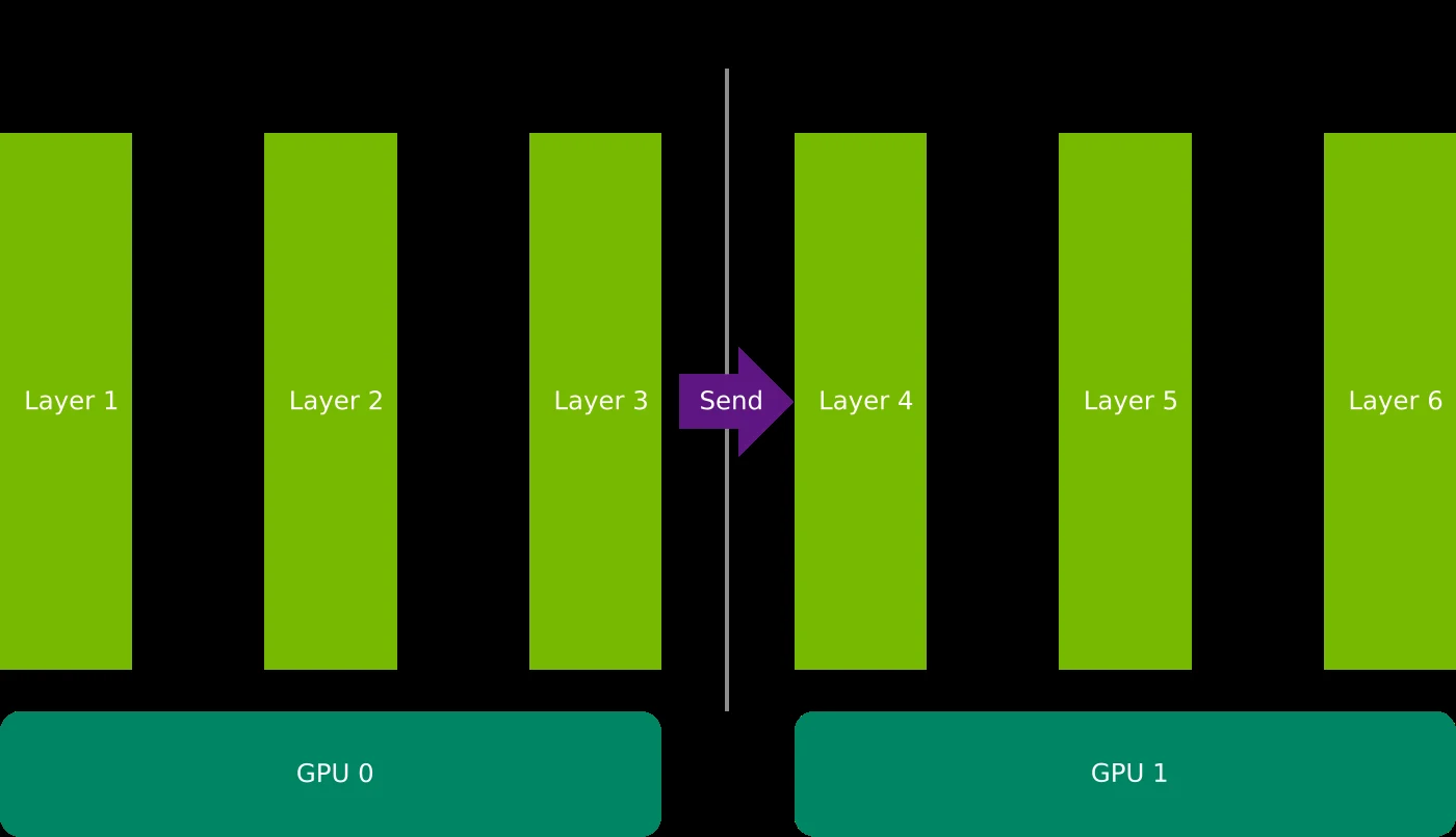
图源:TensorRT-LLM 官方文档(docs/source/media/Pipeline_Parallel_Vis.svg)。图中的横轴是时间、纵轴是 PP 阶段,每个色块是一次 microbatch 的前向;阶段之间的箭头对应下面要讲的 PPCommNCCL.send/recv。
PPCommNCCL 直接建了一个”世界通信子”(world communicator),而不是为每个 PP 组各建一个。为什么可以这么简化?因为 PP 的发送目标是确定的:从 pp_rank 到 pp_rank + 1,对应的全局 rank 可以通过 next_pp_rank 算出来。用世界通信子 + 点对点 send/recv 就足够了,不需要建 per-group 的通信子。
init_pp_comm 里有一大段关于通信子复用的注释,讲的是一个真实的生产问题:
def init_pp_comm(mapping): """Initialize PPComm once at startup""" global _pp_comm if mpi_disabled(): _pp_comm = PPCommTorch(mapping) elif isinstance(_pp_comm, PPCommNCCL) and \ _pp_comm.mapping.world_size == mapping.world_size: # Reuse the existing world NCCL communicator across LLM instances that # share the same worker processes (e.g. a reused MpiPoolSession). The # underlying comm depends only on (world_size, rank) -- it is a world # communicator, independent of the pp/tp/ep layout -- so only the # routing mapping needs refreshing. Recreating it would drop the old # comm and trigger a collective ncclCommDestroy at an unsynchronized # point during the next model build, which can deadlock on reused # workers. ... _pp_comm.mapping = mapping else: if _pp_comm is not None: logger.warning( "init_pp_comm: replacing existing PP comm (world_size " f"{_pp_comm.mapping.world_size} -> {mapping.world_size}) on a " "live process; this can deadlock on reused MPI workers.") _pp_comm = PPCommNCCL(mapping) init_helix_cp_comm(mapping)三个分支的逻辑:
- 复用分支:
world_size相同时只换 mapping 引用,不重建通信子。理由是底层 NCCL communicator 只取决于(world_size, rank),与 pp/tp/ep 的具体布局无关。而重建会触发ncclCommDestroy,这是一个集合操作,在 worker 复用场景下会在未同步的时间点执行,导致死锁。 - 替换分支:
world_size变了,不得不重建,但至少打一条 warning 把风险暴露出来,而不是静默挂住。 - 新建分支:首次调用,正常建。
这类注释在 TensorRT-LLM 源码里不少,它们记录的是”踩过的坑”——读源码时这类段落的价值往往高于主逻辑,因为它解释了为什么不能写成更简洁的形式。
AllReduce:一次通信要经过几层选择
前面讲的是”通信对象怎么来”,现在进入数据面本身。tensorrt_llm/_torch/distributed/ops.py 里的 AllReduce 模块是整条链路上最重要的组件,它的 __init__ 是一棵策略选择树:
class AllReduce(nn.Module):
def __init__(self, mapping: Mapping, strategy: AllReduceStrategy = AllReduceStrategy.AUTO, dtype: Optional[torch.dtype] = None): super().__init__() self.mapping = mapping self.workspace = None self.strategy = strategy self.mnnvl_allreduce = None self.symm_mem_allreduce = None self._disable_mpi = mpi_disabled()
self.all_reduce_op = torch.ops.trtllm.allreduce_pg if self._disable_mpi \ else torch.ops.trtllm.allreduce注意 all_reduce_op 的选择:Ray 模式(mpi_disabled())走 allreduce_pg,MPI 模式走 allreduce。两个 custom op 的区别在于传递通信对象的方式——前者传 ProcessGroup 句柄,后者走 MPI 路径。
可用的策略列表(tensorrt_llm/functional.py 里的 AllReduceStrategy):
class AllReduceStrategy(IntEnum): NCCL = 0 MIN_LATENCY = 1 UB = 2 AUTO = 3 ONESHOT = 4 TWOSHOT = 5 LOWPRECISION = 6 MNNVL = 7 NCCL_SYMMETRIC = 8 SYMM_MEM = 9 # PyTorch symmetric memory with MULTIMEM逐个解释它们在做什么:
| 策略 | 机制 | 适用场景 |
|---|---|---|
NCCL | 直接调 NCCL all-reduce | 通用兜底,跨机也能用 |
MIN_LATENCY | 自定义低延迟 kernel | 小消息(decode 阶段单个 token) |
UB | user-buffer based all-reduce kernel | NVLink 域内,走 IPC buffer |
ONESHOT | 一次全交换,所有 rank 互写 | 消息小、rank 数少 |
TWOSHOT | reduce-scatter + all-gather 两段 | 消息大、rank 数多 |
LOWPRECISION | 传输前降到低精度 | 只有 PCIe 交换机、无 NVLink 的拓扑 |
MNNVL | 多节点 NVLink 多播 | GB200 NVL72 这类跨节点 NVLink 域 |
NCCL_SYMMETRIC | NCCL 的对称内存窗口 | 配合 GEMM 零拷贝 |
SYMM_MEM | PyTorch 对称内存 + MULTIMEM 指令 | SM90/SM100 特定 world size |
AUTO | 按启发式自动选 | 默认 |
AllReduce.__init__ 里对 SYMM_MEM 的处理有一段完整的降级逻辑:
if self.strategy == AllReduceStrategy.SYMM_MEM: try: symm_mem = SymmetricMemoryAllReduce( self.mapping, dtype=dtype if dtype else torch.bfloat16, ) if not symm_mem.disabled: self.symm_mem_allreduce = symm_mem logger.info( f"SymmetricMemoryAllReduce (MULTIMEM) is enabled with fallback support for world_size={self.mapping.tp_size}" ) else: logger.info( "SymmetricMemoryAllReduce is disabled (not supported or unavailable), falling back to AUTO strategy" ) self.strategy = AllReduceStrategy.AUTO except Exception as e: logger.info( f"Symmetric Memory AllReduce can't be enabled due to {e}, falling back to AUTO strategy" ) self.symm_mem_allreduce = None self.strategy = AllReduceStrategy.AUTO注意 except Exception 是故意的:MULTIMEM 是硬件能力,不同 SM 版本、不同 world size 支持情况都不同,探测失败是常态而非异常。把”能力探测”包在宽异常里、失败就退回 AUTO,是这类硬件特性代码的正确写法。注释里那句 with fallback support 也很关键——即使 SYMM_MEM 建成了,workspace 仍然要分配,因为融合算子(fusion_op != NONE)走不了对称内存路径:
if self.strategy != AllReduceStrategy.UB: if self.strategy == AllReduceStrategy.LOWPRECISION: allocate_low_presicion_allreduce_workspace(self.mapping) if self.strategy not in (AllReduceStrategy.UB, AllReduceStrategy.NCCL, AllReduceStrategy.NCCL_SYMMETRIC): self.workspace = get_allreduce_workspace(self.mapping)这段条件判断本身读起来有点绕,但它精确表达了三件事:
UB不需要 workspace(用的是 user buffer)。NCCL和NCCL_SYMMETRIC不需要 workspace(NCCL 自己管缓冲)。- 其余策略都需要 workspace,包括
SYMM_MEM——因为 SYMM_MEM 只能处理fusion_op == NONE,一旦有融合就得走普通路径。
MULTIMEM 的硬件约束
SymmetricMemoryAllReduce(symm_mem_allreduce.py)的类 docstring 直接把支持范围写了出来:
class SymmetricMemoryAllReduce(nn.Module): """ AllReduce implementation using PyTorch's symmetric memory operations. This leverages MULTIMEM hardware instructions for faster allreduce operations.
Supported configurations (world_size): - SM 9.0: 4, 6, 8 GPUs - SM 10.0: 6, 8 GPUs """
# World sizes that support MULTIMEM instructions _WORLD_SIZES_MULTIMEM = { "9.0": [4, 6, 8], "10.0": [6, 8], }以及一组按 SM 版本和 world size 区分的大小上限:
MiB = 1024 * 1024 # Maximum buffer sizes for symmetric memory (bytes) _MAX_SIZES = { "9.0": { 2: 64 * MiB, # 64 MB 4: 32 * MiB, # 32 MB 6: 64 * MiB, 8: 64 * MiB, }, "10.0": { 2: 8 * MiB, # 8 MB 4: 32 * MiB, 6: 128 * MiB, 8: 128 * MiB, }, }为什么 world_size 只能是 4/6/8?因为 MULTIMEM 是走 NVLink 多播(multicast)硬件的——一次写操作同时落到多个 GPU 的显存里。多播组的规模受限于交换机拓扑(NVSwitch 的端口分组),4/6/8 正好对应几种常见的域划分。超出这个范围,要么没有硬件路径,要么收益不足以覆盖开销,所以直接声明不支持。
_MAX_SIZES 的存在则是因为多播缓冲区是预分配的对称内存:world size 越大,每张卡要预留的窗口越多,总占用按平方级增长。SM 9.0(Hopper)和 SM 10.0(Blackwell)的数值不同,反映的是两代 NVLink 交换能力的差异——Blackwell 在 world_size 8 时能给到 128 MiB,而 Hopper 只有 64 MiB。
workspace 大小怎么算
CustomAllReduceHelper.max_workspace_size_auto(allreduce_helper.py)的 docstring 把 workspace 的用途和容量算法讲得很清楚:
@staticmethoddef max_workspace_size_auto(tp_size: int, support_deterministic=True) -> int: """Calculate workspace size for allreduce fusion kernel.
The workspace is used for lamport buffers in the fusion kernel. Required size calculation: - Each GPU needs 3 sub-buffers (for triple buffering) - Each sub-buffer stores: max_num_tokens * hidden_size * dtype_size (bf16=2) - The lamport allocation multiplies by tp_size, so: lamport_size = 3 * size * tp_size (per GPU)
Example: Llama 8B (hidden=4096), max_tokens=8192, bf16, TP=4 - Data per sub-buffer: 8192 * 4096 * 2 = 64 MiB - Total lamport: 3 * 64MB * 4 = 768 MiB per GPU - Required 'size' parameter: 64 MiB (gets multiplied by tp_size in allocation) ... """这段注释值得停下来算一遍。Lamport buffer 是自定义 all-reduce kernel 里用于 rank 间同步的机制——每张卡往自己的 buffer 里写、再读别人的 buffer,不需要 NCCL 的 barrier。三个 sub-buffer 是三缓冲(triple buffering),让写下一批和读上一批能重叠。
按注释里的例子:max_num_tokens = 8192、hidden_size = 4096、bf16,单个 sub-buffer 是 MiB。乘 3(三缓冲)再乘 tp_size(每张卡要持有所有 rank 的 buffer 才做得了本地归约),一张卡要 768 MiB。这不是小开销——用显存换通信延迟就是自定义 all-reduce 的本质取舍。
实际分配时(allocate_allreduce_fusion_workspace):
@staticmethoddef allocate_allreduce_fusion_workspace( mapping: Mapping, size: int) -> Tuple[List[IpcMemory], "torch.tensor"]: is_p2p_supported = can_access_peer(mapping) ipc_buffers_size = size * mapping.tp_size ipc_buffers = IpcMemory(mapping, ipc_buffers_size, is_p2p_supported) ipc_barriers = IpcMemory(mapping, 256 * mapping.tp_size, is_p2p_supported) lamport_buffers_size = size * mapping.tp_size lamport_buffers = IpcMemory(mapping, 3 * lamport_buffers_size, is_p2p_supported) if is_p2p_supported: lamport_initialize(lamport_buffers.local_ptr, 3 * lamport_buffers_size) # flag_buffer[0], atomic flag read counter # flag_buffer[1], non-lamport flag # flag_buffer[2], lamport flag flag_buffer = torch.tensor([0, 0, 0], dtype=torch.int, device="cuda") # layout_buffer[0], clear size for next lamport kernel # layout_buffer[1], triple buffer offset for lamport kernel layout_buffer = torch.tensor([0, lamport_buffers_size], dtype=torch.int64, device="cuda") ...五个组成部分,每个都有明确用途:
ipc_buffers:数据缓冲区,大小size * tp_size。ipc_barriers:同步屏障,每 rank 256 字节。lamport_buffers:三缓冲的 Lamport 区,大小3 * size * tp_size——与注释里的公式严格对应。flag_buffer:三个 int,注释直接给出了各自的语义(原子读计数、非 lamport 标志、lamport 标志)。layout_buffer:两个 int64,记录”下一轮 lamport kernel 要清多少字节”和”三缓冲当前偏移”。
can_access_peer(mapping) 决定这些 buffer 是否能用 P2P 直访(NVLink/P2P 可用时,GPU 之间可以直接读写对方的显存;不可用时只能走主机内存中转)。lamport_initialize 只在 P2P 可用时调用——Lamport 协议的初始化(把 buffer 填成特定的哨兵值)本身要通过 P2P 完成。
默认大小:
# Default: 64 MiB - supports most common model configurations # Increase via env var if you see CUDA illegal memory access errors with large models default_size = 67_108_864 # Exactly 64 MiB return default_size64 MiB 恰好对应注释例子里的”hidden=4096 × max_tokens=8192 × bf16”。注释里那句”遇到 CUDA illegal memory access 就调大”是经验之谈——workspace 不够时报的不是”空间不足”,而是内核越界访存,因为 kernel 会按 layout_buffer 里的偏移去写。这个排查线索很实用。
非确定性的开关
def force_all_reduce_deterministic(): return ( os.getenv("FORCE_DETERMINISTIC", "0") == "1" or os.getenv("FORCE_ALL_REDUCE_DETERMINISTIC", "0") == "1" )以及它对应的处理:
if force_all_reduce_deterministic() and support_deterministic: workspace_size = os.getenv("FORCE_ALLREDUCE_KERNEL_WORKSPACE_SIZE", "1000000000") return int(workspace_size)为什么自定义 all-reduce 会非确定?因为它的归约顺序取决于各 rank 的到达时间——Lamport 协议允许”谁先到谁先写”,浮点加法不满足结合律,顺序不同结果就不同。开启确定性模式后,用更大的 workspace(默认 1 GB)换取固定顺序的归约。这条开关在需要复现实验或对拍数值时会用到。
融合算子:把 all-reduce、残差、归一化、量化压进一次访存
标准 Transformer 的残差块在 TP 下长这样:
h = h + attn_out # 残差相加h = rms_norm(h) # 归一化而 attn_out 是行并行层的输出,需要先 all-reduce。串起来就是三件事:all-reduce → 加残差 → RMSNorm。如果逐个算子做,数据要进出显存三趟:all-reduce 写一遍、加残差读写一遍、归一化读写一遍。以 hidden=8192、bf16、batch 1024 token 计,每次就是 MiB 的读写,乘以三趟和层数就是可观的开销。
TensorRT-LLM 的做法是把它们融成一个 kernel。融合模式的枚举定义在 functional.py:
class AllReduceFusionOp(IntEnum): NONE = 0 RESIDUAL_RMS_NORM = 1 LAST_PROCESS_FOR_UB = 2 RESIDUAL_RMS_PREPOST_NORM = 3 RESIDUAL_RMS_NORM_QUANT_FP8 = 4 RESIDUAL_RMS_NORM_QUANT_NVFP4 = 5 RESIDUAL_RMS_NORM_OUT_QUANT_FP8 = 6 RESIDUAL_RMS_NORM_OUT_QUANT_NVFP4 = 7 MOE_FINALIZE_ALLREDUCE_RESIDUAL_RMS_NORM = 8 RMS_NORM = 9按用途分四组理解:
NONE:纯 all-reduce。- 归一化类:
RMS_NORM(只归一化,不做残差)、RESIDUAL_RMS_NORM(加残差再归一化)、RESIDUAL_RMS_PREPOST_NORM(pre/post 双归一化,某些模型结构需要)。 - 量化类:带
QUANT_FP8/QUANT_NVFP4后缀表示归一化之后直接量化输出。OUT_QUANT_*与不带OUT的区别在于输出的是”归一化结果 + 量化结果”还是只有量化结果——AllReduce.forward的 docstring 把这组返回值的顺序写得很明确:
NONE: [hidden_states]RMS_NORM: [hidden_states]RESIDUAL_RMS_NORM: [hidden_states, residual]RESIDUAL_RMS_NORM_QUANT_FP8: [norm_quant, residual]RESIDUAL_RMS_NORM_OUT_QUANT_FP8: [norm, norm_quant, residual]RESIDUAL_RMS_NORM_QUANT_NVFP4: [norm_quant_fp4, scale_factor, residual]RESIDUAL_RMS_NORM_OUT_QUANT_NVFP4: [norm, norm_quant_fp4, scale_factor, residual]这个”返回几个张量、顺序是什么”的表格是接这条路径时最容易出错的地方。特别是 NVFP4 那条:多出一个 scale_factor——因为 NVFP4 是块量化格式,每 16 个元素共享一个 FP8 缩放因子,缩放因子必须跟着数据一起产出。
MOE_FINALIZE_ALLREDUCE_RESIDUAL_RMS_NORM:MoE 专用,把”专家输出归约 + 共享专家相加 + all-reduce + 残差 + 归一化”五件事合成一个 kernel。这是整个融合体系里最激进的一条,下面单独讲。
融合的载体是 AllReduceParams:
class AllReduceParams:
def __init__( self, strategy: AllReduceStrategy = AllReduceStrategy.AUTO, fusion_op: AllReduceFusionOp = AllReduceFusionOp.NONE, bias: Optional[Tensor] = None, residual: Optional[Tensor] = None, norm_weight: Optional[Tensor] = None, scale: Optional[Tensor] = None, norm_pre_residual_weight: Optional[Tensor] = None, eps: float = 1e-06, enable_allreduce: bool = True, trigger_completion_at_end: bool = True, ): ... assert fusion_op in (AllReduceFusionOp.NONE.value, AllReduceFusionOp.RMS_NORM.value) or (residual is not None)最后那个 assert 是一条契约:只要融合模式涉及残差,就必须传 residual。原因很直观——残差加法的输入不给,kernel 就算不出来。把它写成 assert 而不是运行期检查,是因为这个错误只可能来自模型定义代码写错,属于开发期就该暴露的问题。
还有三个小工具方法:
def has_affine(self): return 1 if self.norm_weight is not None else 0
def has_bias(self): return 1 if self.bias is not None else 0
def has_scale(self): return 1 if self.scale is not None else 0它们把”参数是否为空”编码成 kernel 的模板参数或标志位。这样同一个 kernel 二进制可以覆盖”有/无 bias”、“有/无 scale”两种变体,不需要各编译一份。
AllReduce.forward:策略是分层回退的
forward 的执行路径是一条逐层回退链,值得按顺序读:
def forward(self, input, *, all_reduce_params=None): if self.mapping.tp_size == 1 or (all_reduce_params is not None and all_reduce_params.enable_allreduce == False): return input
input = input.contiguous() # Underlying op requires contiguous input
allreduce_strategy = self.strategy
if all_reduce_params is None: all_reduce_params = AllReduceParams()
# Try Symmetric Memory AllReduce first if available if self.symm_mem_allreduce and all_reduce_params.fusion_op == AllReduceFusionOp.NONE: symm_mem_output = self.symm_mem_allreduce(input) if symm_mem_output is not None: return symm_mem_output elif self.symm_mem_allreduce and all_reduce_params.fusion_op != AllReduceFusionOp.NONE: logger.debug_once( f"Skipping SymmetricMemoryAllReduce for fused operation (fusion_op={all_reduce_params.fusion_op}), using regular allreduce", key=(self.mapping.tp_rank, all_reduce_params.fusion_op, "debug_fusion_skip"), )
# Try MNNVL AllReduce if symm_mem didn't handle it if self.mnnvl_allreduce: mnnvl_output = self.mnnvl_allreduce(input, all_reduce_params=all_reduce_params) if mnnvl_output is not None: return mnnvl_output
# Fall back to regular AllReduce if allreduce_strategy in (AllReduceStrategy.MNNVL, AllReduceStrategy.SYMM_MEM): allreduce_strategy = AllReduceStrategy.AUTO ...四条关键信息:
第一,短路条件有两个。tp_size == 1 是显然的;enable_allreduce == False 则是给上层用的开关——比如 HELIX CP 的注意力输出投影会传 AllReduceParams(enable_allreduce=False),因为在那种布局下它要改用 reduce-scatter,而不是 all-reduce。这比”用两个不同的类”要轻。
第二,contiguous() 不是可有可无的。底层 custom op 按连续内存做向量化访问,非连续输入会直接算错或者报错。注释写明了是为了”满足底层 op 的要求”。
第三,SYMM_MEM 只覆盖 NONE,遇到融合就跳过。原因是 MULTIMEM 是硬件多播指令,只做”把数据同时写到多个 GPU 并求和”这一件事,没法在里面插一段 RMSNorm。代码用 debug_once 记录跳过原因,而不是每次调用都打日志——这种”只打一次”的日志模式在热路径代码里很常见。
第四,策略名会被”改写”:
if allreduce_strategy in (AllReduceStrategy.MNNVL, AllReduceStrategy.SYMM_MEM): allreduce_strategy = AllReduceStrategy.AUTO注释解释得很直接:底层的 allreduceOp 里没有 MNNVL/SYMM_MEM 的分支,所以走到普通路径时必须先把策略名换掉,否则会被判为非法策略。这是一类很典型的”两层策略命名空间不重合一”的问题——上层策略是给”选择逻辑”用的,下层策略是给”kernel 分发”用的。
最后是分发:
if allreduce_strategy == AllReduceStrategy.AUTO and not disable_allreduce_autotune and not self._disable_mpi: if _ALLREDUCE_AUTOTUNER_TUNING_MODE or not _ALLREDUCE_NATIVE_AUTOTUNER_ENABLED: output = torch.ops.trtllm.tunable_allreduce(...) else: output = torch.ops.trtllm.autotuned_allreduce(...) else: output = self.all_reduce_op(...)AUTO 策略下会在开跑时自动调优:tunable_allreduce 会在首个 batch 上试跑几种 kernel 变体,选最快的那个,然后把结果缓存下来供后续批次直接查表(autotuned_allredcüce 走的是查表路径)。这解释了为什么 TensorRT-LLM 的第一次推理往往比后续慢一点——首轮包含 autotune 的开销。
环境变量 TLLM_DISABLE_ALLREDUCE_AUTOTUNE=1 可以关掉这个自动调优(注释里写着是因为曾经观察到性能回退,留了后门)。
GEMM 与 all-reduce 的零拷贝融合
前面提到的 use_fused_gemm_allreduce/NCCL 窗口两条路径,开关条件写在 Linear._refresh_fused_gemm_allreduce 里:
enabled = all([ self.reduce_output, not mpi_disabled(), self.dtype in (torch.float16, torch.bfloat16), self.in_features % 128 == 0, self.out_features % 64 == 0, self.tp_mode == TensorParallelMode.ROW, self.tp_size > 1, quant_valid, get_sm_version() >= 100, self._enable_gemm_allreduce_fusion, os.environ.get("TRTLLM_GEMM_ALLREDUCE_FUSION_ENABLED", "0") == "1",])self.use_fused_gemm_allreduce = enabled and ipc_nvls_supported()十一个条件逐个看,就是一份”这条路径为什么难做”的清单:
reduce_output+ROW+tp_size > 1:必须是行并行且需要归约的层。dtype in (fp16, bf16):低精度才有融合的意义(FP32 通信量太大,融合收益不明显)。in_features % 128 == 0、out_features % 64 == 0:kernel 的 tile 边界要求。quant_valid:要求量化配置里激活也是 NVFP4/FP8 量化的(quant_config_has_nvfp4_activation_quantization)。因为融合路径最终要把 GEMM 的输出直接写进通信缓冲,如果后续还要做量化,必须一并考虑。get_sm_version() >= 100:Blackwell 及以上。这条路径依赖新硬件的特性。ipc_nvls_supported():需要有 NVLS(NVLink SHARP)支持,因为要跨卡直接写多播缓冲。- 一个环境变量开关
TRTLLM_GEMM_ALLREDUCE_FUSION_ENABLED默认关闭。
默认关闭这一点很值得注意:这类”极致优化”的路径在成熟产品里通常先以 opt-in 形式发布,经过充分验证再默认打开。读源码时看到 os.environ.get(...) == "1" 这类默认关闭的开关,基本可以判断这是一条实验性/高风险的路径。
对应的 forward 分支也有注释解释为什么某些情况必须绕开:
if self.tp_mode == TensorParallelMode.ROW: use_locality_domain = self.partition_plan.enabled # The fused GEMM-allreduce and NCCL-window GEMM paths consume the # module's full weight tensors. locality domain releases those tensors after # creating localized shards, so ROW-TP must first run the shard-aware GEMM # and then all-reduce its partial output. use_fused_gemm_allreduce = (not use_locality_domain and self.use_fused_gemm_allreduce and lora_params is None)两个互斥条件:locality domain(把权重按局部性重新分片的技术,会释放完整权重张量)和 LoRA(需要额外注入低秩分支)都会破坏融合路径的前提,所以直接短路。
关于 gather_output 的 sizes:
self.gather_output_sizes = Noneif self.gather_output and self.tp_size > 1 \ and self.tp_mode == TensorParallelMode.COLUMN: if self._tp_sharding_is_auto: sizes = [ end - start for start, end in ( ... ) ]当启用不均匀 TP(uneven TP)时,输出维不能被 tp_size 整除,每张卡的宽度不同。此时 all-gather 必须显式传 sizes,否则按等长切片拼接会错位。同一逻辑在 allgather 的 docstring 里也有:
If 'sizes' is 'None', the input tensors in the different ranks must have the same shape.Otherwise, 'sizes[i]' must be 'input.shape[dim]' at rank i, and the input tensors inthe different ranks can only differ in shape at dimension `dim`.MoEAllReduce:五算子融合
MoE 层的后处理比稠密层更复杂。一个 MoE 层的输出要经过:专家输出按路由权重求和 → 加上共享专家的输出 → all-reduce(TP 部分和)→ 加残差 → RMSNorm。五步。
MoEAllReduce(ops.py)的 docstring 用 torch 参考实现把这条流水线写清楚了:
class MoEAllReduce(nn.Module): """... Notes: * min latency mode:
Support pattern: MoE Reduction + Add + AR + ADD_RMS, see this torch reference implementation: expert_reduction = torch.sum(active_experts_token_input * scale.unsqueeze(-1), dim=0) output_add = expert_reduction + shared_expert_output output_residual = output_add + residual output_hidden_states = rms_norm(output_residual, norm_weight, eps)
* regular mode:
Support pattern: MoE Reduction + Add + AR + ADD_RMS, see this torch reference implementation: expert_reduction = local_reduction(input, expanded_idx_to_permuted_idx, expert_scale_factor) output_add = expert_reduction + shared_expert_output output_residual = output_add + residual output_hidden_states = rms_norm(output_residual, norm_weight, eps) """MoE Reduction 这一项在两模式下不一样,这是关键差异:
- min latency 模式:
expert_reduction是”激活专家输入 × 路由权重、按专家维求和”——也就是说,输入张量已经是”每个 token 每个专家一份”的展开形态,直接在 kernel 里做加权归约。 - regular 模式:
local_reduction(input, expanded_idx_to_permuted_idx, expert_scale_factor)——输入是 permute 过的布局,需要借助expanded_idx_to_permuted_idx(反向索引表)才能把属于同一个 token 的各专家输出归拢起来。
对应的两个 custom op:
if all_reduce_params.is_cutlass_min_latency: return torch.ops.trtllm.moe_allreduce( active_experts_token_input=input, residual=all_reduce_params.residual, norm_weight=all_reduce_params.norm_weight, device_num_experts=all_reduce_params.device_num_experts, scale_input=all_reduce_params.expert_scale_factor, token_input=all_reduce_params.shared_expert_output, workspace=self.workspace, rank=self.mapping.tp_rank, nranks=self.mapping.tp_size, eps=all_reduce_params.eps, )else: if all_reduce_params.residual is not None: assert all_reduce_params.residual.shape[0] <= self.max_token, \ "Num tokens must be less than or equal to max_token"
return torch.ops.trtllm.moe_finalize_allreduce( input=input, residual=all_reduce_params.residual, norm_weight=all_reduce_params.norm_weight, expanded_idx_to_permuted_idx=all_reduce_params.expanded_idx_to_permuted_idx, shared_expert_output=all_reduce_params.shared_expert_output, expert_scale_factor=all_reduce_params.expert_scale_factor, workspace=self.workspace, rank=self.mapping.tp_rank, nranks=self.mapping.tp_size, eps=all_reduce_params.eps, )MoEAllReduce.__init__ 里有一行必须留意的注释:
self.workspace = get_allreduce_workspace(self.mapping)# Pls keep this value in sync with the kOneShotMaxToken in moeAllReduceFusionKernels.hself.max_token = 128这是一个跨语言(Python ↔ CUDA C++)必须手工同步的常量。Python 侧用它做断言,C++ 侧 moeAllReduceFusionKernels.h 里的 kOneShotMaxToken 决定 kernel 的静态形状。两边不一致的后果是:Python 放行了、kernel 越界。注释用”Pls keep this value in sync”这样的措辞直接把约束写在代码里,这是分布式系统里跨层常量维护的常见做法。
is_valid() 则把两种模式的参数依赖显式化:
def is_valid(self): if self.is_cutlass_min_latency: return (self.device_num_experts is not None and self.expert_scale_factor is not None and self.shared_expert_output is not None) else: return self.expanded_idx_to_permuted_idx is not Noneforward 开头的 assert all_reduce_params.is_valid() 因此能挡住”模式选对了但参数没给全”这类错误。
上下文并行的两条路:Ulysses 与 HELIX
到目前讲的都是 TP 和 MoE 的通信。上下文并行(Context Parallel,CP)是长上下文场景下绕不开的一块——当序列长度到 128K、256K 时,KV Cache 本身就把单卡显存吃满,必须沿序列维切开。
mapping.py 里的 CpType 只有三个取值:
class CpType(StrEnum): # CP type for ulysses parallelism ULYSSES = "ULYSSES" # CP type for ring attention RING = "RING" # CP type for helix parallelism HELIX = "HELIX"三者代表了三种截然不同的切分哲学:
Ulysses(DeepSpeed-Ulysses,2023)的做法是沿注意力头维度切分。每张卡持有全部序列但只算一部分头。问题是 QKV 投影的输出是按头切分的,而序列维没切——所以通信模式是:本地算完 QKV 后,用 all-to-all 把”每头一段序列”重排成”每卡一段序列上的所有头”,在本地做注意力,再用一次 all-to-all 换回来。
Ring Attention(2023)则是沿序列维切分,每张卡持有全部头但只有一段序列。注意力需要每个 query 看到全部 KV,所以各卡把自己那段的 KV 沿环传递一圈,边传边累加部分注意力结果。通信量正比于 KV 大小,但用 P2P 环传递,不需要 all-to-all。
HELIX 是 TensorRT-LLM 自己的方案(后面 init_helix_cp_comm 与 HelixCpMnnvlMemory 都是为它服务的),它的核心洞察在前面的 repurpose_helix_cp_to_tp 已经露出来了:CP 只对注意力层有意义,其余层不需要沿序列切。所以同一批卡在注意力层做 CP、在 FFN 层做 TP,把 CP 的”分片”在非注意力部分重新解释成 TP 的分片。这样既不浪费算力,又避免了”CP 组内的卡在 FFN 阶段闲置”。
Ulysses 的 alltoall 与组约束
回到前面那条约束:
if attn_cp_size != 1 and cp_type == CpType.ULYSSES: raise ValueError( f"attn_cp_size must be 1 for now for ulysses, but got {attn_tp_size}, {attn_cp_size}.")现在能解释得更清楚了。Ulysses 的 all-to-all 是在”TP 组 ∪ CP 组”这个合并集合上做的——因为要交换的既有头维度(TP 切的)又有序列维度(CP 切的)。如果允许 attn_cp_size != 1,就意味着注意力层要把这个合并集合再拆,all-to-all 的参与方就变成了一个不完整的集合,语义直接崩掉。所以直接禁止。
HELIX 的注意力:_helix_post_process 与 all-to-all
tensorrt_llm/_torch/attention/attention.py 里有一组以 _helix_ 开头的函数,专门处理 HELIX 的注意力通信。
先看输出的投影:
def _helix_cp_output_projection( o_proj: Linear, attn_output: torch.Tensor, attn_metadata: AttentionMetadata, all_reduce_params: Optional[AllReduceParams], mapping: Mapping, mapping_o: Mapping, layer_idx: int, lora_params: Optional[dict] = None,) -> torch.Tensor: """Apply output projection with reduce-scatter when Helix CP+DP is active.
Reduce-scatter sums partial sums across the CP group and scatters the result so each CP rank processes a distinct token chunk through the MLP. Falls back to the standard AllReduce path otherwise. """ if mapping.has_cp_helix() and mapping.enable_attention_dp: attn_output = o_proj( attn_output, all_reduce_params=AllReduceParams(enable_allreduce=False), lora_params=lora_params, layer_idx=layer_idx)
attn_output, _ = _helix_cp_pad(attn_output, attn_metadata.num_tokens, mapping.cp_size) attn_output = reducescatter(attn_output, mapping_o, dim=0) else: attn_output = o_proj(attn_output, all_reduce_params=all_reduce_params, lora_params=lora_params, layer_idx=layer_idx)
return attn_output关键在于这两行的组合:
attn_output = o_proj(attn_output, all_reduce_params=AllReduceParams(enable_allreduce=False), ...)attn_output = reducescatter(attn_output, mapping_o, dim=0)先做 GEMM 但不做 all-reduce,再用 reduce-scatter 替掉 all-reduce。为什么这样更好?
标准做法是 GEMM → all-reduce,每张卡最后都拿到完整结果。而这里要的是”每张卡只保留自己那一份 token 的结果”——因为下一个 MLP 层也要沿 token 维切分(这正是 attention DP 的语义)。reduce-scatter 一次操作同时完成”归约”和”分发”:把各卡的 partial sum 求和,再把结果按 token 段切给各卡。相比 all-reduce + 后续再切,省掉一次完整的广播。
这就是 enable_allreduce=False 那个开关的真实用途——它不是”关掉通信”,而是”把通信换成另一种形式”。
配套的 _helix_cp_pad 负责对齐:
def _helix_cp_pad(tensor: torch.Tensor, num_tokens: int, cp_size: int) -> tuple[torch.Tensor, int]: """Pad tensor along dim-0 so its length is divisible by cp_size.""" chunk_size = math.ceil(num_tokens / cp_size) padded_size = chunk_size * cp_size ...reduce-scatter 要求各 rank 拿到的段长相等(除非显式传 sizes),所以 token 数必须先补齐到 cp_size 的整数倍。补齐之后各段长度就是 chunk_size,正好是均分的。
再往上看输入侧:
def _helix_cp_allgather_input(hidden_states: torch.Tensor, attn_metadata: AttentionMetadata, mapping: Mapping, layer_idx: int) -> torch.Tensor: """AllGather hidden states from CP group for layers after the first.
The first layer already has the full input from the embedding. Subsequent layers need to undo the previous layer's reduce-scatter. """ if (mapping.has_cp_helix() and mapping.enable_attention_dp and layer_idx > 0): hidden_states = cp_allgather(hidden_states, mapping, dim=0) hidden_states = hidden_states[:attn_metadata.num_tokens] return hidden_states这段注释把整个 HELIX CP + DP 的数据流讲清楚了:reduce-scatter 让每张卡在层末只剩自己那段 token;下一层的注意力需要完整序列才能算(因为注意力是全序列可见的),所以层首要 all-gather 把序列拼回来。
于是每一层的模式是:
[层首] all-gather(拼回完整序列)→ 注意力 → o_proj → reduce-scatter(切回本地 token 段)一层里一 gather 一 scatter,取代了标准 TP 的”一次 all-reduce”。注意 [:attn_metadata.num_tokens] 这个切片——前面 _helix_cp_pad 补过零,gather 回来要切掉填充部分。
模型首尾还要各补一次:
def maybe_slice_for_helix_cp(tensor, attn_metadata, mapping_with_cp, layer_idx): """Slice a tensor to this CP rank's chunk after reduce-scatter.
For the first decoder layer, the residual comes from the embedding and has not been through a prior reduce-scatter. This function slices it so it aligns with the reduce-scattered attention output. ... """ if (mapping_with_cp is not None and mapping_with_cp.has_cp_helix() and mapping_with_cp.enable_attention_dp and layer_idx == 0): tensor, chunk_size = _helix_cp_pad(tensor, attn_metadata.num_tokens, mapping_with_cp.cp_size) start = mapping_with_cp.cp_rank * chunk_size tensor = tensor[start:start + chunk_size] return tensor
def maybe_allgather_for_helix_cp(hidden_states, attn_metadata, mapping_with_cp): """Restore full token count after the last layer's reduce-scatter.
With Helix CP + Attention DP, each decoder layer's reduce-scatter leaves each CP rank with only its chunk of tokens. This function performs an AllGather across the CP group so that the LM head (and final norm) see every token. """ if (mapping_with_cp is not None and mapping_with_cp.has_cp_helix() and mapping_with_cp.enable_attention_dp): hidden_states = cp_allgather(hidden_states, mapping_with_cp, dim=0) hidden_states = hidden_states[:attn_metadata.num_tokens] return hidden_states第一层的残差要对齐:第一层的残差来自 embedding,还是完整序列(没经过上一层的 reduce-scatter),必须手工切到本 rank 的段,才能和已经 scatter 过的注意力输出相加。最后一层之后要 all-gather 回来:LM head 需要看到所有 token 才能出 logits。这两处是最容易漏掉的边界处理——漏掉第一层会 shape 不匹配报错,漏掉最后一层会静默丢掉一部分 token 的输出。
HELIX 的 all-to-all:两种实现
注意力内部本身也要交换数据。HELIX 下每个 CP rank 只算了一段序列上的注意力,但注意力的 softmax 归一化需要全局的 softmax 统计量(最大值和指数和),否则各段单独 softmax 之后拼起来是错的。所以需要一次 all-to-all 把各段的 partial output 和 softmax 统计量换到一起。
_helix_post_process(attention.py)有两条实现路径:
def _helix_post_process(...): ... if <NCCL path>: _helix_note_nccl_specialization(partial_o, softmax_stats, mapping.cp_size) chunks = _helix_nccl_pre_alltoall(partial_o, softmax_stats, zero_kv_mask, mapping.cp_size) gathered = alltoall_helix(chunks, mapping.cp_group) gathered = _helix_nccl_post_alltoall(gathered) return torch.ops.trtllm.helix_post_process(gathered[0], gathered[1], ...) else: helix = HelixAllToAllNative.get(mapping) cp_size = mapping.cp_size ... partial_o_out, softmax_stats_out = helix.alltoall_native(partial_o, softmax_stats, ...) return torch.ops.trtllm.helix_post_process_native(...)NCCL 路径:先 _helix_nccl_pre_alltoall 做数据重排(transpose + split,把”每段的数据”整理成 all-to-all 要的分组形态),调 alltoall_helix(一个用 NCCL send/recv 组实现的 all-to-all),再 _helix_nccl_post_alltoall 把结果整理回需要的布局,最后进 helix_post_process 融合 kernel。
alltoall_helix(ops.py)的 docstring 把接口契约写得很清楚:
def alltoall_helix(inputs: List[torch.Tensor], group: List[int]) -> List[torch.Tensor]: ''' Add an operation that performs a collective all-to-all across a given group. The operation is implemented using a torch op that wraps a NCCL group call of a series of NCCL send/recv operations to implement the all-to-all. ... Args: inputs (List[Tensor]): The input tensors. Its length must be a multiple of the group size, and all tensors in a group must have the same shape. All input tensors must be contiguous. group (List[int]): The group of ranks to participate in the all-to-all. Returns: The output tensors. For each group of input tensors (of size group size), there is one output tensor with shape (group size, *input shape). ''' n_ranks = len(group) if n_ranks == 1: return inputs
assert n_ranks > 0, "group must be non-empty" assert n_ranks == len(set(group)), "group must be unique"
assert len(inputs) % n_ranks == 0,\ "inputs length must be a multiple of the group size" num_lists = len(inputs) // n_ranks for il in range(num_lists): ref_input = inputs[il * n_ranks] assert all([inputs[i].shape == ref_input.shape for i in range(il * n_ranks + 1, (il + 1) * n_ranks)]),\ "all input tensors in a group must have the same shape"
return torch.ops.trtllm.alltoall_helix(inputs, group, num_lists)注意为什么用 NCCL send/recv 而不是 dist.all_to_all:PyTorch 的 all_to_all 要求所有 rank 的输入输出形状一致,而这里要交换的是”partial_o(形状含 kv_lora_rank)“和”softmax_stats(形状含 2)“两种不同的张量,而且 MLA 的 latent 维度在不同 rank 上不总是一致。用 NCCL 的 group call 把一串 send/recv 打包成一个集合操作,既满足了形状灵活性的要求,又保持了”一次 group 调用”的效率。
native 路径(HelixAllToAllNative)则走 MNNVL 内存:
class HelixAllToAllNative: """ Manager for Helix All-to-All operations with MNNVL workspace management.
Exchanges data along the cp_size dimension: - partial_o: [..., cp_size, kv_lora_rank] half-precision - softmax_stats: [..., cp_size, 2] float32 """
# Global cache: mapping -> instance _cache: Dict[Mapping, "HelixAllToAllNative"] = {}
@staticmethod def get(mapping: Mapping) -> "HelixAllToAllNative": if mapping not in HelixAllToAllNative._cache: logger.info(f"Rank {mapping.cp_rank} initializing HelixCpMnnvlMemory for Helix") MnnvlMemory.initialize()
# Get workspace size (in bytes) workspace_size_per_rank = _tllm_internal.thop.get_helix_workspace_size_per_rank( mapping.cp_size)
# Allocate MNNVL memory using CP communicator for Helix workspace = HelixCpMnnvlMemory(mapping, workspace_size_per_rank) workspace_tensor = workspace.as_torch_strided_tensor(torch.uint64)
torch.ops.trtllm.initialize_helix_workspace(workspace_tensor, mapping.cp_rank, mapping.cp_size) torch.cuda.synchronize() HelixCpMnnvlMemory.get_comm(mapping).barrier()
HelixAllToAllNative._cache[mapping] = HelixAllToAllNative( mapping, workspace, workspace_tensor)
return HelixAllToAllNative._cache[mapping]初始化序列里有几个必须注意的点:
- workspace 大小是从 C++ 侧问的(
_tllm_internal.thop.get_helix_workspace_size_per_rank(cp_size))。为什么不硬编码?因为 workspace 布局(每 rank 的段数、偏移)是 kernel 内部的知识,让 C++ 侧统一提供尺寸才不会两边不一致。 initialize_helix_workspace之后要torch.cuda.synchronize(),再做 barrier。这个顺序不能颠倒:workspace 初始化是 GPU 上的操作,必须等它真正完成,才能让所有 rank 确认”大家的 workspace 都就绪了”。少了 synchronize,barrier 可能在 GPU 还在写的时候就放行。_cache是类级全局字典,键是Mapping(同样依赖Mapping.__hash__)。
alltoall_native 的 docstring 里有一条很实用的契约:
def alltoall_native(self, partial_o, softmax_stats, zero_kv_mask=None): """ ... zero_kv_mask: Optional bool mask over the entry dimension, True where this rank owns no KV. The sender rewrites those rows to a no-op contribution, so the caller must not sanitize them itself. """zero_kv_mask 的处理责任在发送方,调用方不要自己清理。注释用”the caller must not sanitize them itself”这种祈使句,说明这个设计曾经有过两种实现并存的混乱。语义上:某些 rank 因为序列切分可能一段 KV 都没有(比如序列很短而 cp_size 很大),这些 rank 的 partial_o 是无效的;但它们的 softmax 统计量(最大值、指数和)必须用”恒等元”参与全局归约——最大值用 、指数和用 。让发送方统一改写,比让每个调用点自己判断更不容易出错。
MNNVL:把显存映射到整个 NVLink 域
前面反复出现 MNNVL 这个词,它值得单独一节。MNNVL(Multi-Node NVLink)指的是跨节点的 NVLink 域——GB200 NVL72 这样的系统里,72 张 GPU 通过 NVLink 交换机连成一个大域,GPU 之间可以直接做显存级访存,不需要经过网络栈或主机内存。
MnnvlMemory(mnnvl_memory.py)是 TensorRT-LLM 对这个能力的封装:
class MnnvlMemory: """MNNVL memory management for tensor parallel (TP) operations."""
# Shared across all subclasses (global/device state). initialized: bool = False fabric_page_size: int = 1 << 29 # 512 MB. dev_id: int = None force_fabric_handle: bool = Falsefabric_page_size = 512 MB 是一个值得停留的数字。NVLink 域内存(fabic memory)的分配粒度远大于普通显存——普通 cudaMalloc 的粒度是 2 MB 量级,而 fabric handle 的粒度是 512 MB。这意味着即使只需要 1 MB 的共享缓冲,也要占掉 512 MB 的地址空间。
这条约束直接影响了前面所有 workspace 的尺寸选择:为什么默认 workspace 是 64 MiB 而不是更小?为什么 _MAX_SIZES 是按 world size 分档的?都是在这个粒度下权衡的结果。
每子类独立的状态
MnnvlMemory.__init_subclass__ 是一段值得学习的 Python 元编程:
def __init_subclass__(cls, **kwargs): """Auto-initialize per-class attributes for each subclass to avoid sharing state with parent.""" super().__init_subclass__(**kwargs) for attr, default in cls._per_class_attrs.items(): if callable(default): setattr(cls, attr, default()) # e.g., dict() creates a fresh dict. else: setattr(cls, attr, default)配合那份 _per_class_attrs 字典:
_per_class_attrs = { "current_mem_offset": 0, "current_rank_stride": 0, # stride for ranks and also address space size. "current_start_address": 0, # Rank count the current address range was reserved for; see # new_mnnvl_memory_address() and _address_window_fits(). "current_address_comm_size": 0, "comm": None, # MPI communicator. # Parallel layout "comm" was split for; see comm_layout_signature(). "comm_signature": None, "allocated_map": dict, # callable for fresh dict. "address_refcnt": dict, # callable for fresh dict. "allocation_granularity": 0,}为什么需要这个:MnnvlMemory 有多个子类(CftMnnvlMemory、HelixCpMnnvlMemory),每个子类管的是不同用途的 NVLink 域内存。如果这些状态变量定义在父类上,两个子类会互相污染——HELIX 的 workspace 偏移会影响到 CFT 的地址分配。用 __init_subclass__ 为每个子类复制一份独立状态,是 Python 里实现”类级实例变量”的标准手法。
current_address_comm_size 和 comm_signature 这两项的存在揭示了一个更深的问题:地址空间预留与通信子必须共同管理。NVLink 域内存一旦预留了一段地址范围,就声明了”这段地址服务于几个 rank”。如果后续并行布局变了(比如从 8 卡变 4 卡),旧的预留就不适用了,必须重新预留。
能力探测:support_nvlink
def support_nvlink(dev_id: int, need_all_up: bool = True): # Do not rely on other modules having initialized NVML as an import side effect. MnnvlMemory._ensure_nvml_initialized() handle = pynvml.nvmlDeviceGetHandleByIndex(dev_id) link_count = pynvml.NVML_NVLINK_MAX_LINKS active_links = 0 available_links = 0 rejected_links = 0 for link_idx in range(link_count): try: if not pynvml.nvmlDeviceGetNvLinkCapability( handle, link_idx, pynvml.NVML_NVLINK_CAP_P2P_SUPPORTED ): continue # NVML_NVLINK_MAX_LINKS is an upper bound over all architectures # and the capability query answers for every index within it. # Only the state query rejects the indices past this GPU's own # link count, so a link counts as available once its state reads. is_active = pynvml.nvmlDeviceGetNvLinkState(handle, link_idx) except (pynvml.NVMLError_NotSupported, pynvml.NVMLError_InvalidArgument): rejected_links += 1 continue available_links += 1 if is_active: active_links += 1 supported = ( active_links == available_links and available_links > 0 if need_all_up else available_links > 0 ) logger.info( f"[MnnvlMemory] dev {dev_id} NVLink: {active_links}/{available_links} links up " f"({link_count - rejected_links} of {link_count} link indices accepted by the driver), " f"need_all_up={need_all_up}, supported={supported}" ) return supported这段代码里最值得学的是注释解释的那个 NVML 行为差异:NVML_NVLINK_MAX_LINKS 是所有架构的上界常量(比如 18),而不是当前 GPU 的链接数。对于链接数少于这个上界的 GPU,遍历到越界索引时:
- 能力查询(
nvmlDeviceGetNvLinkCapability)对越界索引仍然会回答(返回”不支持 P2P”); - 状态查询(
nvmlDeviceGetNvLinkState)对越界索引会抛异常。
所以代码用”状态查询是否成功”来界定”这个索引是否属于本卡的链接”。如果反过来写(用能力查询判断),所有越界索引都会被当成”支持但不活跃的链路”,active_links != available_links 恒成立,探测永远失败。
need_all_up=True 的语义是”全部链路都要起来才算支持”。这是保守策略:只要有链路 down 了,就走不了完整的多播路径,降级到普通 all-reduce 更安全。
supported = ( active_links == available_links and available_links > 0 if need_all_up else available_links > 0)注释里那句”Do not rely on other modules having initialized NVML as an import side effect”也值得注意——显式的初始化依赖,而不是假设别人已经初始化过。这在库代码里是很重要的纪律。
MNNVL all-reduce 的确定性
MNNVLAllReduce 的 docstring:
class MNNVLAllReduce(nn.Module): """A specialized AllReduce implementation for Multi-Node NVLink communication. ... The oneshot kernel is deterministic across ranks. For TP sizes up to 8, it uses a rank-specialized fast path that keeps the local value in registers and volatile-loads only peers from the Lamport buffer. Larger world sizes use a compact deterministic fallback. ... """两点信息:
- one-shot kernel 是跨 rank 确定性的。这与前面自定义 all-reduce 需要
FORCE_ALL_REDUCE_DETERMINISTIC开关的情况不同——MNNVL 的 one-shot 天然确定。原因在于它的做法:把本地值留在寄存器里,只对 peer 的数据做 volatile-load。也就是说归约顺序被固定成”本地值 + rank 0 + rank 1 + …”,不依赖到达顺序。 - TP ≤ 8 有专门的快速路径,更大的 world size 走”紧凑的确定性兜底路径”。8 这个界限对应 NVSwitch 域的常见划分。
类里还有一组类级字典管理 workspace 生命周期:
allreduce_mnnvl_workspaces: typing.ClassVar[dict[Mapping, _MnnvlWorkspace]] = {}
# Workspaces a larger one replaced after a CUDA graph capture used them. Those graphs still launch on their buffers # and flags, so they stay alive with the process. The checkpoint hooks cover only the current workspace. allreduce_mnnvl_retired_workspaces: typing.ClassVar[dict[Mapping, list[_MnnvlWorkspace]]] = {}
# Communicators split for a mapping whose workspace construction has not # succeeded yet. Ownership moves to the workspace once it is published, so # an entry here is never reachable from allreduce_mnnvl_workspaces. allreduce_mnnvl_pending_comms: typing.ClassVar[dict[Mapping, _MpiCommProtocol]] = {}
# The guard makes lock creation atomic, while each mapping lock serializes # its complete workspace construction and publication lifecycle. _allreduce_mnnvl_workspace_locks: typing.ClassVar[dict[Mapping, threading.Lock]] = {} _allreduce_mnnvl_workspace_locks_guard: typing.ClassVar[threading.Lock] = threading.Lock()allreduce_mnnvl_retired_workspaces 的存在理由写得很清楚:CUDA Graph 捕获时会记录 kernel 用的缓冲区指针。如果后来因为需要更大空间换了新 workspace,旧缓冲区不能释放——已捕获的 graph 仍然会往那块地址写。所以旧的 workspace 被”退休”到一个单独列表里,随进程存活。这是一个非常 GPU-specific 的陷阱:CUDA Graph 的捕获把内存地址固化进了执行图,任何”重新分配”的优化都必须考虑这一点。
_allreduce_mnnvl_workspace_locks_guard 则是一个经典的 double-checked locking 结构:用一个全局锁保护”每 mapping 一把锁”的字典本身,每把 mapping 锁再串行化该 mapping 的 workspace 构建与发布。注释里”makes lock creation atomic”说的正是这个。
MNNVL 支持哪些融合
SUPPORTED_FUSION_OPS: frozenset[AllReduceFusionOp] = frozenset({ AllReduceFusionOp.RMS_NORM, AllReduceFusionOp.RESIDUAL_RMS_NORM, AllReduceFusionOp.RESIDUAL_RMS_NORM_QUANT_FP8, AllReduceFusionOp.RESIDUAL_RMS_NORM_QUANT_NVFP4, AllReduceFusionOp.RESIDUAL_RMS_NORM_OUT_QUANT_FP8, AllReduceFusionOp.RESIDUAL_RMS_NORM_OUT_QUANT_NVFP4, })六种融合模式,全部围绕 RMSNorm。对比一下 AllReduceFusionOp 的全部取值,这里面少了 NONE、LAST_PROCESS_FOR_UB、RESIDUAL_RMS_PREPOST_NORM、MOE_FINALIZE_ALLREDUCE_RESIDUAL_RMS_NORM。也就是说 MNNVL 路径不处理 MoE 那个五算子融合。
这类”支持矩阵”用 frozenset 声明、在运行时检查,是硬件路径代码的标准写法——能力边界显式化,而不是让调用方去猜。
一次多卡前向的完整通信图
把前面的内容拼起来。以 8 卡、tp_size=4, cp_size=2, pp_size=1、跑一个 MoE 模型(moe_tp_size=2, moe_ep_size=4)、开启 attention DP 为例,一次 decode step 里的通信活动是:
注意力层(HELIX CP + DP 模式)
- 层首
cp_allgather:把各 CP rank 的 token 段拼回完整序列(_helix_cp_allgather_input,layer_idx > 0才需要)。 - 注意力内部
alltoall(原生 MNNVL 或 NCCL send/recv 组):交换 partial output 与 softmax 统计量。 - 输出投影
o_proj走enable_allreduce=False,随后reducescatter:把结果切回本地 token 段。
FFN / MoE 层
- 专家路由的 all-to-all:token 按路由结果在
moe_ep_group(这里是[0,1,2,3]或[4,5,6,7])内分发。 - 专家计算后
MoEAllReduce:五算子融合(专家归约 + 共享专家 + all-reduce + 残差 + RMSNorm),走moe_finalize_allreduce或moe_allreduce。
层间
- TP 组内(这里
[0,2,4,6]和[1,3,5,7])所有行并行层的 all-reduce——如果use_fused_gemm_allreduce成立,这一次搬运被省掉,GEMM 直接写进通信缓冲。
模型首尾
- 第一层残差切片对齐、最后一层后
cp_allgather让 LM head 看到全部 token。
一张图看清各组的关系:
8 卡,tp=4, cp=2, pp=1
全局 rank: 0 1 2 3 4 5 6 7cp_rank: 0 1 0 1 0 1 0 1tp_rank: 0 0 1 1 2 2 3 3pp_rank: 0 0 0 0 0 0 0 0
CP 组: [0,1] [2,3] [4,5] [6,7] ← 连续,机内 NVLinkTP 组: [0,2,4,6] [1,3,5,7] ← 步长 2,交错
MoE (moe_tp=2, moe_ep=4, cluster=1):MoE EP 组: [0,1,2,3] [4,5,6,7] ← all-to-all 走这里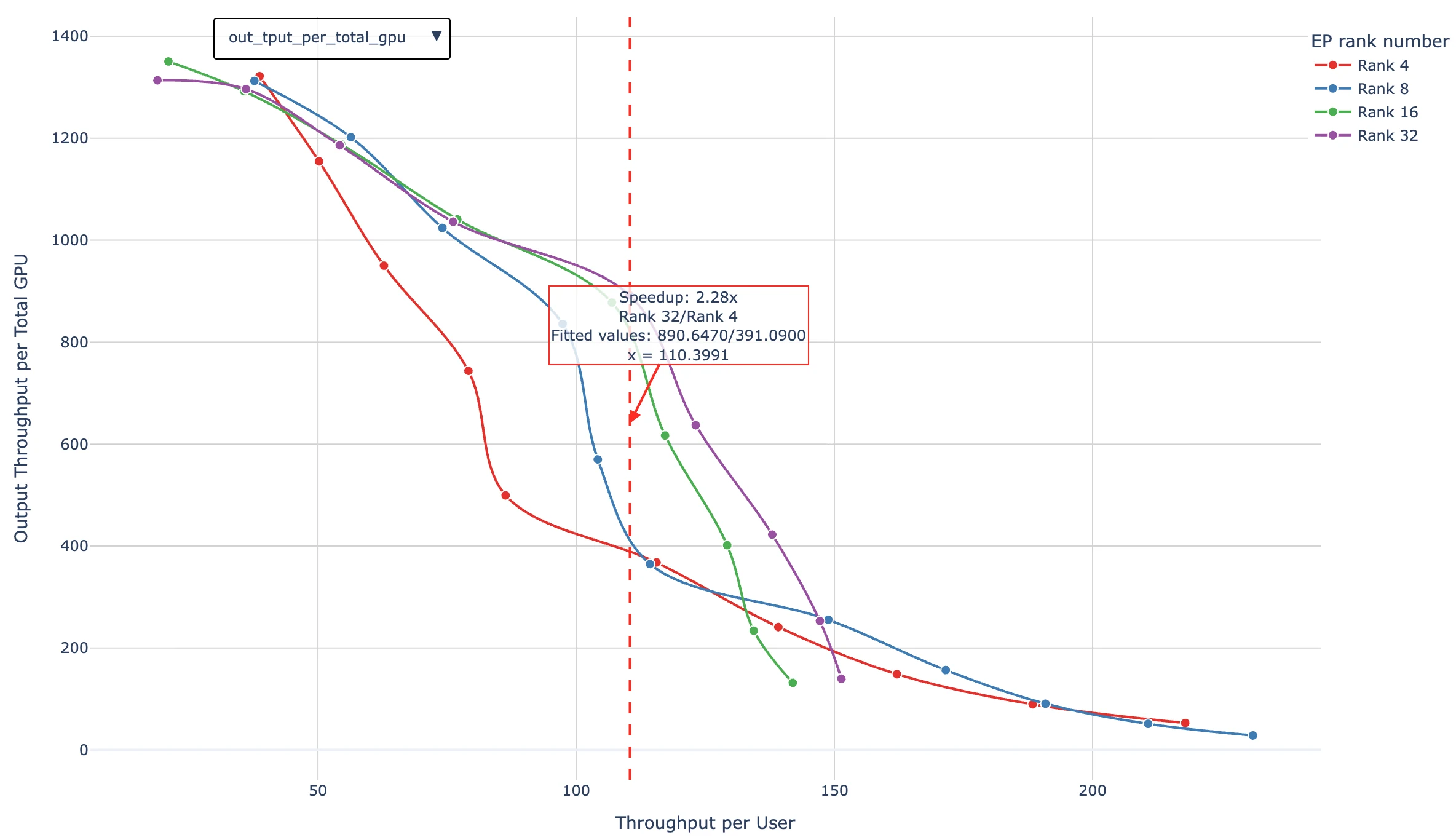
图源:TensorRT-LLM 官方技术博客(`docs/source/blogs/media/tech_blog15_ds32_wide_ep.png`)。这张图是把前面的小型拓扑表放大到真实部署规模后的样子:EP 组不再是 4 个 rank,而是几十上百个 rank 组成的一整个专家并行域,DP Attention 组与 EP 组的边界也不再重合。它同时也是理解"为什么需要把 cluster 与 EP 分开建模"的最好例子——规模一大,跨 cluster 的 all-to-all 就会变成主导开销。
MoE TP 组: [0,4] [1,5] [2,6] [3,7]这张图也解释了为什么 MpiTopology 的 docstring 要把这些组一个个列出来——它们不是”顺便生成”的,每一个都对应一条真实的通信路径。
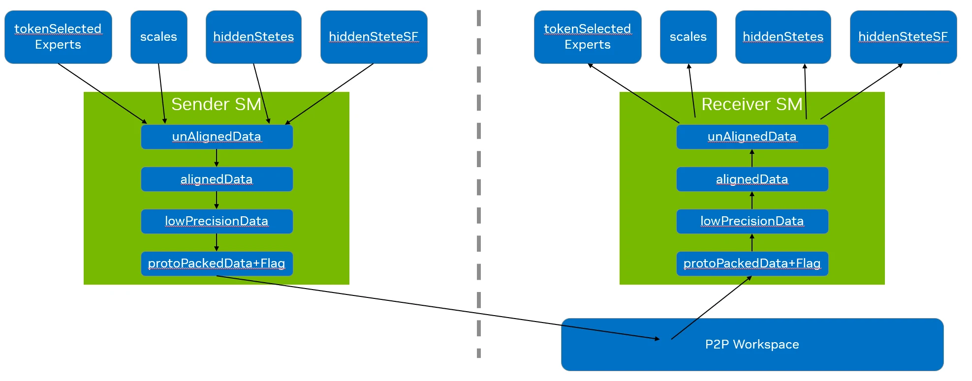
图源:TensorRT-LLM 官方技术博客(docs/source/blogs/media/tech_blog14_alltoall_dataflow.png)。这张图把上一节列出的第 4 步——专家路由的 all-to-all——画了出来:发送侧按路由结果把 token 分组发出,接收侧把收到的 token 拼接后交给本地专家,算完再沿反向路径送回。它与 MoEAllReduce 里的 expanded_idx_to_permuted_idx 是同一套索引的两端。
小结
把这一篇的结论收拢成可以直接记住的几条:
Mapping是一个混合进制坐标系:rank = pp_rank × (tp×cp) + tp_rank × cp + cp_rank,CP 放在最低位让 CP 组连续、落在机内高带宽域。三条乘法等式(tp×pp×cp = world_size、moe_tp×moe_ep×moe_cluster = moe_world_size、attn_tp×attn_cp = tp×cp)定义了整个并行空间的合法性边界。- 组划分与组索引必须成对读:
_init_parallel_groups的四段循环决定组列表的排列顺序,property 里的乘法权重与之严格对应;MoE 的三层嵌套(cluster/EP/TP)让索引公式变长,读法是先画出遍历顺序树。 repurpose_helix_cp_to_tp是 HELIX 的本质:一个进程持有两个Mapping,注意力层当 CP、FFN 层当 TP。- Ray 模式用
init_device_mesh复刻同一套 rank 语义:维度顺序[pp, moe_tp/moe_ep 或 tp, cp],MoE 两维展平成虚拟tp;build_mesh是进程级单例,所以world_size=1的 Mapping 要返回SingleProcessGroup而不是去用作业级网格。 Distributed.get用lru_cache缓存通信对象,键是Mapping——这意味着模型里 N 个Linear层只会建一次进程组,代价是Mapping必须正确实现__hash__。AllReduce的策略选择是一棵带降级的树:SYMM_MEM 探测失败退 AUTO、融合算子跳过 SYMM_MEM、MNNVL/SYMM_MEM 在普通路径上改名成 AUTO、AUTO 走 autotune 查表。每一条降级都在日志里留痕。- 融合是这条链路真正的价值所在:
AllReduceFusionOp把 all-reduce + 残差 + RMSNorm + 量化压进一次访存;MoEAllReduce更进一步把”专家归约 + 共享专家 + all-reduce + 残差 + RMSNorm”五件事合一。返回值顺序(尤其 NVFP4 多出的scale_factor)是接这条路径时最容易出错的地方。 - workspace 是”用显存换延迟”的具体载体:Lamport 三缓冲按
3 × size × tp_size分配,64 MiB 默认值对应 hidden=4096 × tokens=8192 × bf16;空间不够报的是 CUDA illegal memory access 而不是”空间不足”。 - MNNVL 把显存映射到整个 NVLink 域:fabric 页粒度 512 MB 决定了所有 workspace 尺寸的下限;one-shot kernel 天然跨 rank 确定(本地值留寄存器、只 volatile-load peer);
retired_workspaces的存在是因为 CUDA Graph 把缓冲地址固化进了执行图。 - HELIX CP + DP 的层内模式是”all-gather → 注意力 → o_proj → reduce-scatter”:
enable_allreduce=False不是关掉通信,而是把 all-reduce 换成 reduce-scatter,顺带完成 token 段的重新分发;第一层残差要手工切片对齐,最后一层后要 all-gather 回来。
下一篇会继续沿并行主线往下走:注意力层的 QKV 切分与 MLA 在多卡上的布局——即 attn_tp_size/attn_cp_size 如何真正落到 head 维度的分配、MLA 的 latent 表示在 TP 下怎么切、以及这部分与 KV Cache 池的交互。
参考资料
- TensorRT-LLM GitHub 仓库 —— 本文代码引用来自
tensorrt_llm/mapping.py、tensorrt_llm/_torch/device_mesh.py、tensorrt_llm/_torch/distributed/、tensorrt_llm/_torch/modules/linear.py与tensorrt_llm/llmapi/llm_args.py - TensorRT-LLM 官方文档:Parallelism —— TP/PP/CP/EP 的官方配置说明
- DeepSpeed-Ulysses: System Optimizations for Enabling Training of Extreme Long Sequence Transformer Models —— Ulysses 上下文并行的原始论文,all-to-all 按 head 切分的来源
- Ring Attention with Blockwise Transformers for Near-Infinite Context —— Ring Attention 原始论文
- Efficient Memory Management for Large Language Model Serving with PagedAttention —— vLLM 的 PagedAttention,KV Cache 分页管理的来源
- NCCL User Guide: Collectives —— all-reduce、all-gather、all-to-all 的语义与实现说明
- PyTorch Distributed Documentation ——
new_group、ProcessGroup、init_device_mesh的行为约定 - NVIDIA NVLink and NVSwitch —— NVLink 域与多播(MULTIMEM/NVLS)能力的硬件背景
- DeepSeek-V3 Technical Report —— MLA(Multi-head Latent Attention)的 latent 表示与 KV 压缩,HELIX 的
kv_lora_rank来源于此
文章分享
如果这篇文章对你有帮助,欢迎分享给更多人!
评论区
正在获取所在地区…
正在读取天气
音乐
暂未播放